Cold Box Upgrade and Commissioning and temperature analysis of pixel modules

Transcription

1 Cold Box Upgrade and Commissioning and temperature analysis of pixel modules Simon Storz Semester Thesis, ETH Zurich, Institute for Particle Physics IPP Supervisors: Prof. Rainer Wallny, Andrey Starodumov, Felix Bachmair July 31, 2014 Abstract This document describes a Semesterarbeit done at the Institute for Particle Physics IPP at ETH Zürich. It is about commissioning an upgraded cold box which is used to test pixel modules for the CMS detector in it. A step by step guide to calibrate sensor temperature in the box is given. The document contains temperature (and humidity) measurements which show the temperature distribution in the box and on the modules. Furthermore, measurements of the temperature dependency of the leakage current and the DAC parameters of the pixel modules are shown. 1

2 Contents 1 Introduction 3 2 CMS Experiment CMS Detector Silicon Tracker Pixel Modules Setup Cold Box Electronic equipment Readout Cold Box Upgrade 10 5 Measurements Cold Box: Cooling analysis Humidity Temperature Air Base Plate Module Holder Module Comparison Leakage Current Calibration Temperature table DAC temperature dependency Conclusion 27 A Setup 31 A.1 Conductor Board: Circuit diagram A.2 Python codes B Measurements 48 B.1 Humidity and air temperature B.2 Base plate B.3 Module Holder B.4 Leakage current C DAC dependency 59 2

3 1 Introduction This paper is part of a Semesterarbeit done at the Institute for Particle Physics IPP at ETH Zürich. It is part of the Pixel group that works on the upgrade of the CMS pixel detector at the LHC at CERN which is planned for For the upgrade process every redesigned pixel module which will be installed inside the CMS detector has first to be tested. This is where this Semesterarbeit comes into play. Its aim is to upgrade and commission the cold box where inside the modules later will be tested. An electronic set up is developed to measure temperature and humidity and to easily read out the quantities with a python script. This is used to analyse the temperature and humidity in the cold box in detail. Furthermore, the temperature distribution on module holders and of modules itself are measured in various conditions. Finally, the dependence of DAC parameters on the temperature of the silicon is investigated. The important results are shown and explained in this paper, all data and further graphs can be found in the Appendix. 2 CMS Experiment 2.1 CMS Detector The CMS experiment is part of the Large Hadron Collider (LHC) at CERN. The LHC basically consists of two 27 kilometre long underground beam pipes in which hadrons are accelerated to a velocity close to the speed of light and will later collide. One of the collisions is done in the middle of the CMS pixel detector. When two hadrons (composite particles held together by the strong force, consist of quarks) collide, some of the energy gained by the collision is turned into mass, namely new particles. The CMS pixel detector is able to detect these resonances with di erent layers of the detector (figure 1). Most of the particles the scientists are looking for have a very short lifetime when they are created by the energy of the collision. Then they decay in other particles which can be tracked by the detector and give information about the mother-particle (e.g. a Higgs boson) we are looking for. Each of the daughter-particles can be observed in a di erent layer of the detector: For example the energy of the electron e can be measured in the electromagnetic calorimeter (ECAL). A e flying through the ECAL deposits energy in form of photon showers in proportion to the energy of the e. Hadrons are observed in similar manner in the hadron calorimeter. Muons can fly even through the superconducting solenoid which is used to bend the paths of the particles which are about to collide. Muons are detected in the Muon chambers, neutrinos can not be detected at all. Their presence can be recalculated through missing energy and momentum. 2.2 Silicon Tracker The Pixel Detector forms the innermost part of the detector. Its aim is to track the path of the particles which are created in the collision of the two protons. This part of the detector provides the best resolution of the path of the particles. The path is bent by a magnetic field. The reconstruction of its radius gives information about the momentum of the particle which is crucial in order to know which particle was involved 3

4 Figure 1: The CMS detector. in the collision. This way the tracker can reconstruct the paths of electrons, high-energy muons and hadrons as well as short lived decay particles. [1] The pixel detector which is made out of silicon contains 65 million pixels which track the particle s path. There are di erent layers of readout modules containing these pixels. 2.3 Pixel Modules One Pixel Module consists of a electronics layer, base strips, a sensor layer and 16 silicon read out chips, each containing 4160 pixels (figure 2). The silicon sensor is electrically connected to 16 (...) ROCs. The connection between sensor and ROCs is made of indium bumps, which connect each sensor pixel with a pixel unit cell (PUC) on the ROC. On top of the sensor a High Density Interconnect (HDI) serves as an interface to the front end electronics. [4] A charged particle crossing the sensor layer loses energy due to elastic scattering with electrons. Thanks to this energy electron-hole pairs are created in the depleted semiconductor silicon. This causes a small current to flow. These electrons reach the ROCs due to the bias voltage. [4] There the current gets amplified in order that it is enough strong to be measured. [2] At the bottom there are the base strips which are needed to fix the module onto the support. 4

5 Figure 2: One part of a silicon chip (schematic view) with the sensor layer on top of the ROC. 3 Setup All experiments related to this Semesterarbeit will be done in the cold box in the clean room of the ETH Institute for Particle Physics IPP. Figure 3 shows the setup with the cold box on the left, an analogue testboard on the top and a Keithley multimeter which powers the module placed in the box. Figure 3: Experimental setup in the ETH IPP cleanroom. 3.1 Cold Box The following experiments are done in a Cold Box. This is a machine providing thermal control for a particular volume. With the cold box the thermal circumstances of the CMS experiments are simulated. The cold box is controlled by the built in JUMO software. The user can program any cooling cycle with the controller in the box or via USB connection with the supervising 5

6 software elcomandante. Latter is recommended for long term measurements and if the temperature must be held at a particular setpoint until it is stable. The cooling of the cold box is provided by four peltier elements which lie directly underneath the base plate (model: QuickCool QC M 4x4cm). A peltier element consists of two touching semiconductors with di erent conduction band energy levels. When a current flows, one electron has to absorb energy to jump to the higher conduction band of the other semiconductor. This absorbed energy is provided by thermal energy causing one semiconductor to cool down. The other semiconductor which absorbed the electron gets warmer. This is the cooling e ect of the peltier elements. [7] They sit on a copper block in which the water flows. Thanks to the high thermal conductivity of copper, the heat produced by the peltier elements can be dissipated by the water flowing through the block. It is important that the water flow is always on during the cooling process in order not to damage the peltier elements. Additionally, there is a tube which connects the inner part of the cold box with a dry air filter outside the box. Thanks to that the humidity in the box can be controlled by floating or flushing dry air. It is therefore crucial that every part of the box is well sealed so that no humid air can float into the box. The seal is done with foam rubber, tape, and heavy plumb bricks loading the box (see figure 3) so that the cap is tightly shut. 3.2 Electronic equipment For the temperature and humidity measurements explained in the following chapters, PT1000 temperature sensors and Honeywell HIH4020 humidity sensors are used. They are connected to a constant current source (DAC/5V), provided by the Labjack. The Labjack is an interface between measurement devices and a computer. It reads the electrical inputs of a connected sensor and sends this information to the computer. The sensors both work in a similar way: The resistance of the sensors (platinum for PT1000) depends on the temperature respectively the humidity of the material. This causes a voltage drop over the sensor that can be measured by the Labjack. The measurement was done with a4wiremeasurementtoprovidemoreexactresults. All sensors are connected to a conductor board (figure 4) whose design and construction was one part of this Semesterarbeit. It was developed within 3 versions. For the first measurements (everything until chapter 5.2.4) the second version was used which was self built in the electronics laboratory. The new board (figure 4) was built professionally by the ETH electronics team according to the drawing made with the software eagle that is attached in Appendix A.1. On the bottom of the board it can be connected to the Labjack U6, that converts the analogue voltage signal to a number which can be read out with a computer. In the middle of the plate there are two connectors for sensors providing digital readout by the Labjack. In the middle on the top there is a connector for an analogue readout sensor that provides two output channels. One possibility is to connect a Sensirion SHT75 sensor here measuring temperature and humidity simultaneously. The 12 connectors on the edge of the board are meant to connect with PT1000 and HIH4020 humidity sensors (or others as well). In front of each connector is a jointer that is needed to be covered according to the used sensor type. If a humidity sensor is plugged in, the jointer has to be covered with the part where the H (for humidity) is marked. If there is a temperature sensor plugged in, the jointer has to be covered the other way where the 6

7 Figure 4: Conductor board with Labjack T (temperature) is written. This is because the sensors are read out di erently, which will be explained in the next chapter. The design of the board makes it possible to measure 16 channels simultaneously. They are numbered from the left (AIN0) to the right (AIN11) plus the middle sensor (AIN12/13). This can also be seen in the attached circuit diagram (appendix A.1). It can be freely chosen how many of these 16 channels are temperature measurements and how many humidity. As figure 5 shows, the sensors correspond very well: the sensors are stuck very close to each other in the box. Then the temperature (resp. humidity) values of each sensor are compared. The PT1000 sensors used for the measurements correspond very good: they di er by 0.2 C. The humidity sensors di er by 1.5%. This inaccuracy has to be taken into account in the humidity map where the gradient is very small anyway (figure 10). Figure 5: Left: Accuracy of used temperature sensors. Right: Accuracy of used humidity sensors with the corresponding label on the sensor. 7

8 The Labjack provides a voltage readout with an accuracy of ±0.01V. For the old board as well as the new one the resistances of the PT1000 sensors could be read with an accuracy of <1 Ohmwhichis<1 permillandcorrespondstoanaccuracyintemperature of <0.5 C. Therefore these are the most fundamental inaccuracies on every measurement values that will be shown in this paper and this forms the limit to how exact the data can be measured. 3.3 Readout As already mentioned the Labjack connected to the board with a DB37 connector converts the measured voltages of the sensors to a number that can be read out with a computer connected with USB. There is a Python module providing commands for the U6 Labjack. There is a di erence between the readout of temperature and humidity (see figure 6): For! DAC!!!! 5V Pre-Resistance (1000 Ohms)!!!!! PT1000 HIH4020 GND GND Figure 6: Schematic view of the readout of a temperature sensor (above) and a humidity sensor (bottom). humidity, the measured voltage is proportional to the relative humidity with the relation: rh =(V out z)/s (1) where the z=zero o set and s=slope are constants depending on the sensor. With temperature, things are a bit di erent: There we have a DAC which we set to 0.1 V. But we don t know the exact current yet for each sensor. Therefore an additional resistance which is measured very exactly is placed in front of the sensor and the jointer. Thanks to this the current I = R v 0 v can be found. The conversion to resistance goes as follows: R = v R 0 v 0 v (2) with the measured input voltage v, the reference resistance R 0 which lies in front of the particular connector and the reference voltage v 0 which has to be measured at one of the connectors while covering the second and third inlet of the connector. This is the reason 8

9 why the jointer has to be attached correctly in front of every connector depending on the connected sensor. The resistances are converted to temperatures the following way: T = a r a 2 (R 100)/b (3) 2b 4b 2 with R = the measured resistance / 10 and the constants a =3.902e 1andb =5.802e 5 for R>100 and T = ar 5 + br 4 + cr 3 + dr 2 + er + f (4) with R = the measured resistance / 10 and the constants a = , b = , c = , d = , e =2.219 and f = for R<100. This formula is also used to convert the resistances measured by additional sensors read out by a Keithley multimeter. All python codes - also the ones for the plots - are attached in the appendix. 9

10 4 Cold Box Upgrade The first aim is to improve the cold box: The new upgraded box should provide a stronger and faster cooling in order to make it as comfortable as possible to work with for upgraded CMS modules testing. In comparison with the old box several things have changed: 1. First, the diameter of the water tubes are enlarged. The old tubes with a diameter of 9 mm are replaced by others with a diameter of 12 mm (see figure 7). Therefore also the magnetic valve has to be exchanged with one with a larger diameter. Now every part of the box where the water flows has a minimum diameter of 9 mm. Figure 7: Left: The old (left) and new (right) water tubes in comparison. Right: The inside of the cold box. Thanks to the larger tubes, the maximal water flow of the box rises to 33.7 l/min. According to the formula dv dt = v A (5) with the flow rate dv, the velocity v of the water and the cross-section area A, the dt maximal flow of the old box was 18.8 l/h if the box operated with the same water pressure. 2. Second, a new copper block is installed to the Cold Box. Before, there was only one passage of water in the copper block under the base plate of the box. Now water flows through the copper plate in two parallel pipes having opposite directions. 3. Moreover, new peltier elements are built in. They are as large as before (4x4 cm 2 ). Every part of the cooling box is tightened by cellular rubber, styrofoam and tape to avoid humid air getting in and rising the humidity. 10

11 5 Measurements 5.1 Cold Box: Cooling analysis First, the behaviour of the upgraded cold box is investigated. There are 10 cycles programmed for the analysis of the cooling process of the box: In each cycle, the box cools down to -20 Candafterwardsheatsupto+20C while flushing dry air. As figure 8 shows, the temperature rises beyond the +20 Csetpointineachcycle. Thisshowsthatit takes about one minute until the box gets colder again. This is because the material and the air need some time to transport the colder atoms to the JUMO sensor. Moreover the relative humidity always stays between 5 and 10 % and lowers during the multiple cycle process which is a good result for further module testing in the box. Figure 8: 10 temperature cycles in the new Cooling Box Figure 9 shows one cooling process in detail for the setpoint values -20 Cand-25C. The new cold box reaches a stable level of -20 C in 12 minutes and -25 C in 20 minutes. The lowest reachable temperature is C. We see from this results that the upgraded box can cool faster and to a lower temperature than the old box. There it took 16 minutes to cool to -20 C, a cooling to -25 Cwasnotpossible. Figure 9: Cooling to setpoints -20 Cand-25C 11

12 5.2 Humidity Figure 10: Left: Humidity sensors in the cold box. Right: Humidity map for setpoint temperature -25 C. Now the box and the electronic equipment is used to measure thermal quantities of the setup. First we have a look at relative humidity in the cold box. This is measured with Honeywell HIH4010 sensors as seen in figure 10 (left). The sensors are placed 4.5 cm above the base plate, which is 1/3 of the total height of the cold box. Totally 25 points are measured. First, the box is floated with dry air until the Jumo sensor reached a humidity level of 9%. Then the box is cooled down to -25 C. The measurement is started as soon as the temperature in the box is stable. For humidity, 100 measurements are done for each sensor. Then the mean value is taken. The corresponding relative humidity map is pictured in figure 10 (right). The humidity varies by 1.7% within the box. It can be observed that the rearward part has a higher relative humidity than the other parts. First it has to be mentioned that this can not be caused by a particular sensor not working well because the measurements are done row by row (not column by column). There are two possible explanations why the rearward part has a higher relative humidity. First, the sealing between the cap and the base plate could be not perfect, so some humid air may come in there. As the air in the box is colder than the air outside the air pressure outsides is higher. It is estimated that this thermal e ect is stronger than the floating dry air (60l/h) in the box rising the pressure inside. Therefore there is a possibility that there is a small leaking at the rear. The alternative explanation is that the dry air does not float rectangular to the base plate into the box. This small angle causes the air to come to the front part of the box first, causing the more humid air to float to the rearward part. This explanation is consistent with the map of the air temperature shown in the next chapter. In any case a minor redesign of the box should be considered. On the one hand it has to be ensured for future box upgrades that the dry air floats perfectly rectangular into the box. This could be achieved by fixing the air tube better to the base plate and to look that the tube is not bended too strong before the connection to the base plate. On the other hand the mechanism of the cap could be reconsidered. The problem with a 12

13 possible leaking is a common one and could be resolved by changing the way the cap is fastened to the box. Now it is folded from the bottom to the front. The sealing could be improved by tightening the cap to the base plate. This could be done with screws or another tightening mechanism. 5.3 Temperature Air The air temperature in the box is measured simultaneously with the humidity. Therefore, the positions (4.5 cm above the base plate) as well as the initial conditions of the measurements are the same as described above. Figure 11: Left: Temperature map of the air temperature at 4.5 cm above the base plate of the cold box. Right: All measurements of the point in the 4th row from the top, 5th column. No trend can be seen, the measurements fluctuate around a mean value. The air temperature distribution is shown in figure 11. The temperatures are on average 15 Chigherthanonthebaseplateunderneath(setpoint-25 C; see chapter 5.2.2). Delta(T) is 3 C. As figure 11 (right) shows this is a map which is not only valid for a few seconds: The 100 measurements of the points (which took about 3 minutes) fluctuate around the mean value which is shown in the map. This indicates that the situation shown in figure 11 is stable. The standard deviation on the values is apple1.1 C. The white point shows the position where the dry air flows into the box. The mean dewpoint at 4.5 cm height in the box is ±2.2 CaccordingtothemeasurementswiththeLabjack. This corresponds well with the dewpoint calculated from the temperature and humidity value the Jumo sensor measured: Here the dewpoint is ± 1.1 C. The formula for the dewpoint calculation is: y T DP = c (6) b y with y = ln( rh 100 )+b T (7) c + T and b =17.67, c =243.5 C. In addition, it can be seen that the temperatures in the front of the box are much higher than on the other parts. This could again be explained by the 13

14 non rectangular dry air tube. This causes warmer air to flow to the front parts of the box and explains why we measure a low air temperature at the position where the air comes in. Nevertheless, more investigations on the air temperature are recommended Base Plate For this part, the number of measurement points is increased to a 7x7 map of the temperatures on the base plate of the cold box. The PT1000 sensors were stuck to the base plate with thermal paste and tape as shown in figure 12 (left). 150 measurements are done for each sensor. First, the box is flushed with dry air until the Jumo sensor shows a humidity value under 9 %. Then the cooling begins. The measured temperature distribution is what was expected: In the middle parts where the peltier elements are, the coolest temperatures are observed. In the measurement with setpoint -25 C(figure13), the base plate gets here even colder than the setpoint value. From the middle to the left and right border we see that the temperature steadily increases. This e ect is stronger on the right side of the box (delta(t )=6C; left side: delta(t )=5C) and it is stronger at colder setpoint temperatures. These measurements correspond very well with those of Brian Kaputska [5] with the non-upgraded cold box. The standard deviation on the values are apple1.5 C for each measurement point and apple4.2 Cforthepointsinthemiddleon top of the peltier elements. This is a gradient we expect to see. In contrary the delta(t) in the vertical direction is something we want to have as low as possible. It is 0.5 Cat the outer parts and 1.5 Cinthemiddlewherethepeltierelementsare. Thegradientis bigger in the middle because during the 150 measurements which take about 5 minutes the peltier elements do not cool constantly. Their cooling depends on the Jumo sensor which forces them to stop cooling if the temperature falls under the setpoint and vice versa. All in all these are good results: They show that the temperature distribution on most parts of the base plate of the upgraded box is much more homogeneous than within the old box. There a vertical delta(t) of 0.8 C was measured [5]. Figure 12: Left: Temperature measurement on the base plate with 7 PT1000 temperature sensors. Right: Temperature map of the base plate at setpoint -20 C. 14

15 Figure 13: Temperature map of the cold box base plate at setpoint -25 C. The measurement points are marked with crosses. Figure 14: Temperature distribution of the red module holder in the cold box at position 1andsetpointtemperature-25C. 15

16 Figure 15: Left: The 3 tested module holders. Right: Exact measurement of red module holder at module position and position 1 in cold box. Setpoint: -25 C. 16

17 5.3.3 Module Holder In this part we are interested in the temperature distribution on the module holders on which pixel modules later will be tested. For that we make several di erent measurements: First, the temperature of one module holder is measured on every part of the holder. For that, the red module holder (see figure 15 right) is placed on position 1 in the cold box (2nd from the top). Then the box is cooled down to -25 C. Now the temperatures of 21 measurement points on top of the module holder are taken. As the heatmap in figure 14 shows, the total temperature gradient is 5 C. As expected we observe that the coolest part of the module holder is in the middle where the peltier element lies underneath. The temperature gradient between the middle and the outer parts look very similar to the distribution on the base plate (figure 13). The error on the values are apple1.2 C. One has to take into account that the measurement on this particular area of the module holder on the 4 positions in the cold box. Figure 16: Temperature dependence of the yellow base plate is not very exact which explains the more detailed structure of the module holder temperature map. From now on, we concentrate on the part of the module holder where the module will later be placed. We want to compare this area of interest later with other measurements of the module base strips. First, an exact measurement of this part on the red holder is taken (figure 15). No module is installed on the holder. The part we are looking at begins at the module holder length of 2.3 cm and ends at 5.8 cm. We observe a temperature gradient of C in this area. The left part is the warmest, the right border is the coldest. This measurement is done without any other module holders in the box. The temperature on the module holder increases by 1 Cif3other(red)holdersareinsertedintothebox. One could say that the thermal energy in the box is distributed to the three other holders as well causing the first one to cool down a bit. The corresponding heatmap is attached in appendix B.3. 17

18 Next, the temperature dependence on the module holder material and thickness is investigated. So far, all measurements are done with the red holder. We now repeat the temperature measurement of the area where the module later will be installed with the two other other stainless aluminium holders (figure 15 left). The silver holder is 1.15 mm thicker than the others (4.15 mm: silver holder. 3.0 mm: Red and gold holder.). The gold and red holders are anodized. The temperatures on particular positions on the di erent holders vary by 0.5 Cwhichiswithinthestandarddeviationontheindividualtemperature measurements (apple1 C). It can be said that it does not make a significant di erence in temperature if another module holder is used. The detailed color maps are attached in appendix B.3. Finally, it is of great interest whether the temperatures on the module holder di er between the 4 positions in the box. Therefore, the temperatures are measured on the yellow holder on the 4 di erent positions in the box. The results are shown in figure 16. Position 2 is the one with the smallest temperature dependence. All in all a temperature gradient of maximal 1.2 Ccanbeobserved.Theonlypointwithatemperaturegradient of more than 1 Cistheupperrightcorner. Theotherpointsvarywithlessthanthe standard deviation (apple 1 C) on the temperature values which shows that the gradient between the positions is not significant. The temperature distribution on the holder itself reproduces very well the distribution on the base plate which is what we expect to see. The measurements on the module holders also show that there is only a small di erence in the temperature distribution if we change something in the setup (position, holder, insert other holders). This is an important information for the operation of the box and further tests of the pixel modules. Figure 18: Module holder with PT1000 temperature sensor underneath and module on top of it Module In this chapter, the temperature on powered modules are observed. A module is put onto the yellow module holder. In fact for the following experiments, a slightly di erent 18

19 Figure 19: Temperature distribution on module with unpowered ROCs (above) and powered ROCs (below). module holder is used (see figure 18). It has a built in PT1000 temperature sensor which lies underneath the middle of the module and measures the temperature on the bottom of the module. To compare all the measurements later, again a setpoint of -25 Cischosen. Forthefirstpart,the module is powered, but not the ROCs. The temperature is measured on the 6 holders of the base strip of the module, as seen on figure 17. Furthermore, the PT1000 sensor under the module is taken into account. Thus there are totally 7 measurement points. The PT1000 sensors are stuck onto the 6 base strip holders with conductive paste. Then the sensors and therefore the whole module are pressed with captain tape against the module holder. In the second part the ROCs get powered. After waiting about 10 minutes, the second measurement is done. The results red circles represent the measure- Figure 17: CMS Pixel module. The are illustrated in figure 19 and show that the mean ment points of the PT1000 sensors. temperature increases by 1.7 C(errorapple1C) when the ROCs are powered. This is caused by the current heating up the silicon material of the ROCs which heats up the base strips Comparison Now it is possible to compare the di erent steps. We are interested in the temperature distribution of the whole setup. This is illustrated in figure 20. It can be seen that the mean temperature of the base plate and the module holder at the shown position is 19

20 the same, but the temperature gradient on the module holder is much smaller and more homogeneous. From the module holder to the base strips a small temperature increase of 0.4 C is observed. When powering the ROCs we see another temperature increase on the base strips of 1.7 C, which is much higher than the inaccuracies on the temperature values and therefore significant. All in all a mean temperature gradient of 2.1 Cismeasuredon the same position between the base plate and on the module base strips. Figure 20: Comparison of the temperature distribution on a) the base plate at the area of interest b) the important part of the module holder c) the module base strips with unpowered ROCs c) with powered ROCs. All measurements were done under the same conditions, positions and with a setpoint of -25 C Leakage Current The leakage current which powers the module strongly depends on the temperature of the silicon material: I Leakage = I 0 T 2 e E G 1 2k B T (8) with the band gap energy of silicon E G =1.11 ev at T =302K and the calibration constant I 0 which depends on the sensor and the setup. The calibration constant can be found with the sensor calibration which is described later. Here a constant of I 0 =0.018 was found. The calibration constant can also be found more accurate by including the temperature dependency of I 0 : I Leakage = I L,reference T T ref e E G 2k B ( 1 T 1 T ref ) (9) Here, I L,reference is the leakage current measured at a reference temperature (described in chapter 5.3.7) and T ref the corresponding sensor temperature read out with the PT

21 touching the ROCs. This more detailed calculation does not change the results much as figure 22 shows: The slopes of the interpolation lines di er only by All in all it shifts the temperature values by 0.5 Ctolowervalues. First it is of great interest to look at the long-time behaviour of the leakage current at a particular JUMO setpoint. In figure 21 it can be seen that it takes about 5 hours to reach a stable leakage current if the box and the module are set to thermal equilibrium. If the box is set to a particular setpoint, it takes much less time (approx. 20 min) to have a stable leakage current flowing through the module. This is important for the calibration part that will be explained later. After the leakage current has got stable, the current remains constant. Further data is attached in the appendix. Figure 21: Left: Behaviour of the leakage current in thermal equilibrium with unpowered ROCs. Right: Behaviour at a JUMO setpoint of +17 CwithpoweredROCs. Now three temperatures are compared: The one measured by a) the JUMO sensor on the bottom of the cold box base plate b) the ROCs temperature measured by the PT1000 sitting underneath the tested module and c) the sensor temperature which is read out from the leakage current via formula 8 (figure 22). The whole measurement was done twice, giving slightly di erent results. The slopes of the interpolation lines between the two measurements only di er by 0.009, but there is a remarkable shift to lower temperatures (delta(t)=-2.5 C) in the value of the sensor temperature in the second measurement. Such a corresponding shift is also seen on the values of the ROC temperature represented by the PT1000 underneath the module (delta(t)=-1.5 C). The two measurements were done with exactly the same conditions. It is not yet fully understood why the two measurements di er that much. One possibility could be that the module was already working a few hours before the first measurements were done. This could have caused the silicon to be much warmer from the beginning. The second measurement was done on another day where the module has not been used before for several hours. The problem that the leakage current di ers from measurement to measurement is also discussed later in this chapter in correlation with reproducibility. It is important to see that the slopes of the two measurements do not di er much and that the di erence is only caused by a constant shift. Nevertheless the second measurement is preferred because of the explanation above and the fact that it agrees much better with the temperature measurements from chapter than the first measurement. Also shown in figure 22 is the calibration point in green, with which the calibration of formula 8 was done. More graphs can be found in Appendix B.4. The leakage current di ers whether the ROCs are powered or not. As seen before an 21

22 Figure 22: Temperature converted from leakage current, PT1000 underneath the module and JUMO sensor compared at di erent JUMO setpoints. ROCs power on. increase in temperature is observed when the ROCs get powered. This measurement is done with the PT1000 sensors on the base strip. Now similar results can be found for the silicon sensor material by looking at the leakage current (and the converted temperature) of the module at a setpoint of +17 C in the box (figure 23). First, the ROCs are unpowered. Then suddenly the ROCs get powered and the leakage current rises by 7.5*10 8 A. This corresponds to a temperature increase of 2.6 C from 17.1 C to 19.7 C. Comparing these results with the temperature rise of the ROCs it can be seen that this part of the sensor heats up less (+1.4 C) than the silicon which a ects the leakage current. This agrees with the bigger slope of the silicon seen in figure 22. Moreover, it is also observed how good the results from the leakage current measurements can be reproduced. The first part is to start the measurement of the leakage current (JUMO setpoint: +17 C, ROCs powered), wait for 45 minutes, note the measured stable leakage current, and stop the measurement. Then without any setup changes, do the same again. The result of this reproducibility measurement is that the measured leakage current values di er by Awhichcorrespondstoatemperatureof1.05C. The second part is to open the cold box, lift the module holder with the module on it and to put it down again at the same position (1) between each measurement. This is to investigate whether there is an influence on the temperature if the module holder is not perfectly flat and lies di erently on the base plate each time. Here it can be seen that the leakage current di ers by Aeachtime(1.7C). There is one measurement (the first one) which gives much higher results than all other four and was therefore not 22

23 Figure 23: ROCs first unpowered and then powered. Setpoint: +17 C. taken into account in this calculation. Probably something with the module changed after this first measurement, causing all following ones to measure lower currents. The detailed graph can be found in the appendix. The leakage current measurements show that the temperatures of the silicon sensor material is 3.3 C lower than the JUMO sensor and 5.5 Clowerthanthetemperatureof the ROCs at a setpoint of -25 C. In addition it has been shown that one has to wait for 20 minutes until any tests with pixel modules should be started in the cold box, using any particular JUMO setpoint. There it does not have an influence whether the ROCs are powered or not. If the box is set to thermal equilibrium, the leakage current and therefore the sensor temperature needs 5 hours to get stable. This only works for unpowered ROCs as there are breakthroughs of current observed when the ROCs are powered (see Appendix B.4), causing the current to not get stable at all. The results of the sensor temperature measurements are not what was expected to see and are not fully understood yet. They could be observed in more detail in further investigations Calibration After installing a new cold box it is important to calibrate the sensor temperature and the leakage current before measuring anything that has to do with temperature corresponding to the current of the module. This is how to do the calibration: 1. First, the calibration point has to be found. Therefore, a module has to be installed in the cold box. Power the module, but not the ROCs. 2. Close the box and set it to thermal equilibrium: Water flow (33-44l/h), dry air flow (approx. 60l/h), setpoint: 40 C to prevent the peltier elements from cooling. 3. Now track the leakage current and the resistance of the PT1000 underneath the module with elcomandante for some hours (see figure 21 (left)). Therefore the bias voltage has to be set to -150V provided by a Keithley multimeter connected to the testboard. It is important to be sure to have reached a stable thermal equilibrium and therefore a stable leakage current in the box before moving on. Now, the PT1000 temperature under the module and the temperature converted from the stable leakage current should correspond well. We assume that now the ROCs and the sensor 23

24 have the same temperature because they are in thermal equilibrium. The temperature of the PT1000 is read out by another Keithley and tracked with elcomandante. It can later be converted to a temperature. The calibration measurement done for this Semesterarbeit gives the following data: JUMO sensor temperature: C; temperature of PT1000: C; I Leakage =3.65e-7 A. 4. Now the sensor constant in formula 8 can be found inserting the measured leakage current I Leakage and for T the temperature measured by the PT1000 under the module. This gives I From now on temperature conversions from the measured leakage current should be calibrated. This can be tested the following way: turn on the ROCs power. Set several JUMO setpoints between +20 C and-25 C(e.g. steps of 5 C). For each measurement the leakage current is measured and compared with the values of the PT1000 (figure 22). Important: Before each measurement one has to wait until the leakage current gets stable. This takes (see figure 21 right) about minutes Temperature table On the table below the di erent measurements are shown and can be looked up. BP = base plate; MH = module holder; BS = module base strips. The listed measurements with powered modules are all made with ROCs power on. The data of the base strip and module holder measurements show the part where the module sits on (position 1 in the box) as shown in figure 20. The listed base strip temperature data is taken from the corresponding heatmaps and shows the mean values of the left, middle and right part of the area. The temperature gradient is very small in the y direction and only in x direction in this area of the plate. The data of the module holder measurements are mean values of each two measurements (up & below) for the left, middle and right part of the yellow module holder (as shown in figure 15 left) with a detailed measurement of the yellow holder which is attached in the appendix. The values of the base strip temperatures are calculated in the same way as before, but with the data of the measurements in figure 19 (below). The Temperature values of the ROCs of the sensor which are measured by the PT1000 sensor built in the module holder (figure 18) are also listed. Finally the temperatures of the silicon sensor are converted from the leakage current measurement shown in figure 22. The converted temperatures and the leakage current (in Ampere) are listed. It can be seen that when the JUMO sensor of the box shows -25 C, this is also the mean temperature on the position of interest on the base plate. There is no significant temperature gradient between the base plate and the module holder. But there is small one (0.4 C) between the module holder and the base strips. With powered ROCs the gradient is even bigger (approx 2 C). With a setpoint of -25 CthepoweredROCsreach a temperature which is about 2.3 C warmer than the JUMO setpoint. The delta(t) between the JUMO sensor and the sensor material is -3.3 C. JUMO temp BP left BP middle BP right MH l MH m MH r BS l BS m BS r ROCs temp Sensor temp Leakage c > e e e e e-9 24

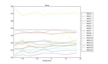
25 5.4 DAC temperature dependency In this chapter the dependence of the DAC parameters on the temperature which control the ROCs is investigated. A module is placed inside the cooling box. With elcomandante, several tests are set: Pretest at 17 C, Pretest at 10 C, Pretest at 0 C, Pretest at -5 C, Pretest at -10 C, Pretest at -15 C, Pretest at -20 C,Pretest at -25 C. In each step, the box cools down until a stable setpoint is reached. Then the pretest optimises the DAC parameters for the corresponding temperature in the box. The data is stored and can later be compared: There are only 5 out of 21 DAC parameters which change with temperature. This can be Figure 24: Left: Behaviour of all 21 DAC parameters of ROC1 after the pretest at di erent temperatures. Right: Mean changes of the 5 interesting DAC parameters of all ROCs. seen in figure 24 left with the behaviour of the ROC1-DAC parameters after the pretest at di erent temperatures. Now we concentrate on the 5 DAC parameters that change with temperature: Vana, VthrComp, Vo setr0, VIrefADC and CalDel. The detailed graphs for these parameters are shown in figure 25. One can see that the distribution among the ROCs is very small for VIrefADC (new name: PHScale) and VO setr0 (new name: PHO set). There are two outliers for ROC0 and ROC12 at +10 Cand-10C which correspond for both parameters. For Vana the values do not change much for different temperatures: There are fluctuations but no significant temperature dependence. AsimilarmeasurementwasdonebyC.Eggelfortheoldmodulesin2009[6](page68) who compared the DAC parameters Vana, VthrComp and CalDel for +17 Cand-10C. The results are shown in figure 24. The two data points of Eggel for Vana indicate a stronger temperature dependence as observed in this experiment. But as there are only two data points one should be carefully interpreting too much in it. The results for the temperature dependence of VthrComp and CalDel show a similar behaviour as the data of Eggel: CalDel gets higher for lower temperatures. VthrComp does not vary much and only shows some fluctuations which agrees with the two data points of Eggel. Interesting is the big range of the observed VthrComp and CalDel values among the ROCs (figure 25). Possibly this has to do with the new Pyxar algorithm which replaced the classical approach of psi46expert. Finally there are big anomalies in the results of the last measurement at -25 C. It can be seen that the values of VIrefADC and VO setr0 are at the upper limit (255) which shows that the pulse height optimization has failed. This could be caused by a not converging algorithm which sets CalDel in the Pretest at -25 Ctoafixedvalue(allROCshavea 25

26 very similar value, see figure 25). There are a few open issues in this chapter. First, more statistics about the temperature dependency of the DAC values for temperatures >-25 Careneeded. Thetests should be reproduced with di erent Pretest algorithms, namely Pxar. Then the measurement at the setpoint of -25 C have to be redone to verify whether the shown data can be reproduced. If this is the case it would lead in the finding that the ROCs are not e cient at -25 C. If a further test shows di erent results at this temperatures it is likely that this particular test done in this Semesterarbeit had a problem here, and that there is no issue with the ROCs at -25 C. Furthermore it would be interesting to have information about the temperature dependency on the Trim parameters. 26

27 Figure 25: Behaviour of the 5 DAC parameters that change with temperature. parameter is shown for every of the 16 ROCs. Each 6 Conclusion Thanks to this Semesterarbeit everyone who needs to work with pixel modules in the cold box profits from the detailed temperature maps of the di erent parts of the setup shown before. It has been observed that the temperature gradient between the cold box base plate and the module base strip is small (apple 1 C). Little changes to the setup (e.g. varying module positions or changing module holders) do not have a big influence on the temperature distributions. The temperature on the base strips are 0.4 C higher than on 27

28 the module holders and the base plate. With powered ROCs the temperature on the base strips are approx. 2 C higher than the temperature on the base plate and the JUMO sensor. With a JUMO setpoint of -25 Cthesensormaterialofthepixelmodulesget C cold and the ROCs are much warmer: They reach a temperature of C. The upgraded cold box provides a faster cooling (12 minutes to -20 C; 19 minutes to -25 C) and can cool down to lower temperatures than before. The changes of this upgrade should be considered for any other cold box. In addition, information was gained about the behaviour of the leakage current at different temperatures. It has been shown that one needs to wait 20 minutes before starting any module test in the cold box after having reached a particular JUMO setpoint. If the box is set to thermal equilibrium, one needs to wait for 5 hours until the leakage current and therefore the sensor temperature gets stable. Moreover, it has been observed that there are five DAC parameters depending on the temperature: Vana, Vo setr0, VIrefADC, VthrComp and CalDel. Big variations have been measured among the ROCs for VthrComp and CalDel. At a setpoint of -25 Cbiganomalieshavebeenfoundindicating that either the module is not e cient at this temperature or the Pretest has failed only in this experiment. Furthermore, a step by step guide how to calibrate the silicon sensor temperature was given which can be used for any future experiments in the cold box. With the chosen method of measuring an accuracy of apple1 Conmostofthemeasurements was reached which was satisfying for the shown experiments. The electronic setup with the conductor board and the sensors can also be used for other applications at the IPP. Some further experiments could expand the knowledge about temperature dependence of pixel modules. First, more experiments concerning the humidity and air temperature in the box would possibly lead to an even stronger proposal to redesign parts of the cooling box. It could also be observed whether the humidity a ects module tests. In addition, there should be more tests done concerning the temperature dependence of the DAC parameters. More data is needed to get a more detailed picture of the dependence and the anomalies at -25 C. Also tests of the temperature dependence of the DAC parameters after Trimming are recommended. All in all this Semesterarbeit gives much information about the temperature and humidity distribution in the cold box, the module testing setup and the modules itself and it lays the foundation of any further investigations in this field. References [1] Lucas Taylor, /05/06 [2] Lucas Taylor, /05/06 [3] Dominguez, A. et al.: CMS Technical Design Report for the Pixel Detector Upgrade. No. CERN-LHCC CMS-TDR-011, [4] Trueb, Peter. CMS pixel module qualification and Monte-Carlo study of H to tau + tau tol + l ET. Diss. Zurich No , U., [5] B. Kapustka, Cooling Box Commissioning Presentation, 2013/02/06 28

29 [6] Eggel, Christina. CMS pixel module qualification and search for B 0 s to mu + mu. Diss. Zurich No , ETH, [7] /22/06 List of Figures 1 The CMS detector. (Source: ) Silicon Chip. Source: Experimental setup in the ETH IPP cleanroom Conductor board with Labjack Left: Accuracy of used temperature sensors. Right: Accuracy of used humidity sensors with the corresponding label on the sensor Schematic view of the readout of a temperature sensor (above) and a humidity sensor (bottom) Left: The old (left) and new (right) water tubes in comparison. Right: The inside of the cold box temperature cycles in the new Cooling Box Cooling to setpoints -20 Cand-25C Left: Humidity sensors in the cold box. Right: Humidity map for setpoint temperature -25 C Left: Temperature map of the air temperature at 4.5 cm above the base plate of the cold box. Right: All measurements of the point in the 4th row from the top, 5th column. No trend can be seen, the measurements fluctuate around a mean value Left: Temperature measurement on the base plate with 7 PT1000 temperature sensors. Right: Temperature map of the base plate at setpoint -20 C Temperature map of the cold box base plate at setpoint -25 C. The measurement points are marked with crosses Temperature distribution of the red module holder in the cold box at position 1 and setpoint temperature -25 C Left: The 3 tested module holders. Right: Exact measurement of red module holder at module position and position 1 in cold box. Setpoint: -25 C Temperature dependence of the yellow module holder on the 4 positions in the cold box Module holder with PT1000 temperature sensor underneath and module on top of it Temperature distribution on module with unpowered ROCs (above) and powered ROCs (below) CMS Pixel module. [3] (page 73)

30 20 Comparison of the temperature distribution on a) the base plate at the area of interest b) the important part of the module holder c) the module base strips with unpowered ROCs c) with powered ROCs. All measurements were done under the same conditions, positions and with a setpoint of -25 C Left: Behaviour of the leakage current in thermal equilibrium with unpowered ROCs. Right: Behaviour at a JUMO setpoint of +17 Cwithpowered ROCs Temperature converted from leakage current, PT1000 underneath the module and JUMO sensor compared at di erent JUMO setpoints. ROCs power on ROCs first unpowered and then powered. Setpoint: +17 C Left: Behaviour of all 21 DAC parameters of ROC1 after the pretest at di erent temperatures. Right: Mean changes of the 5 interesting DAC parameters of all ROCs Behaviour of the 5 DAC parameters that change with temperature. Each parameter is shown for every of the 16 ROCs Code to read out the values from Labjack and convert them tho temperature/humidity Code to create diagrams with leakage current and resistance measurements Code to create heatmaps of the cold box base plate Code to create heatmaps of the module holder Code to create heatmaps of the base strips

31 A Setup 31

32 1 Pretest Sensor Calibration of old sensors 2 Pretest Sensor Calibration of new sensors 3 at setpoint -25 C 4 H Humidity 32

33 A.1 Conductor Board: Circuit diagram 33

34 Circuit diagram of the new circuit board. By Simon Storz, ETH Zürich IPP,

35 35

36 A.2 Python codes 36

37 /Users/simonstorz/Documents/ETH/SemesterThesis/Code/measure Kopie.py Saved: :48:15 Page 1 of 6 Printed For: Simon Storz import u6 import math import numpy as np class test: def init (self): self.d = u6.u6() self.d.getcalibrationdata() self.d.getfeedback(u6.dac1_8(self.d.voltagetodacbits(.1,dacnumber=1,is16bits=false))) self.channels_row1 = [12,4,5,3] self.channels_row2 = [1,0,2,6] self.channelth = -1 self.resistance0oldplate = {1:995.2,3:995.7,5:996.3,0:995.8,2:996.4,4:994.9,6:996.3,8:1102.5} self.resistance0= {0:995.6,1:995.01,2:994.0,3:994.66,4:994.91,5:995.0,6:995.8,7:995.9,8:996.06,9:994. self.hiha = {90:0.8132,92:0.814,93:0.812,94:0.810,95:0.810} self.hihb = {90:0.031,92:0.031,93:0.031,94:0.031,95:0.031} self.hihc = {90:1.0546,92:1.0546,93:1.0546,94:1.0546,95:1.0546} self.hihd = {90: ,92: ,93: ,94: ,95: } self.supplyvoltage =.1 self.channels=[1,2,3,4,5,6,7] self.channels_hih =[7,8,9,10,11] self.hihsensors=[92,95,94,90,93] self.naverage = 150 def del (self): self.d.close() def len (self,a): return len(a) def SetDAC1(self,voltage): self.d.getfeedback(u6.dac1_8(self.d.voltagetodacbits(voltage,dacnumber=1,is16bits=false))) def get_accurate_ain(self,channel,gain=0): feedbackargument = u6.ain24(positivechannel=channel, ResolutionIndex=13, GainIndex=Gain) Figure 26: Code to read out the values from Labjack and convert them tho temperature/humidity 37

38 /Users/simonstorz/Documents/ETH/SemesterThesis/Code/measure Kopie.py Saved: :48:15 Page 2 of 6 Printed For: Simon Storz ainbits = self.d.getfeedback(feedbackargument) v = self.d.binarytocalibratedanalogvoltage(gainindex=gain,bytesvoltage=ainbits[0]) return v return self.d.getain(channel) def measure(self,channel0,channels,rs,nges=10): n= 0 Rges=[] Rges2=[] ri=[] for i in channels: Rges.append(0) Rges2.append(0) for k in range(0,nges): vi = [self.get_accurate_ain(i,1) for i in channels] v0 = self.get_accurate_ain(channel0,1) print 'v0',v0 RT = map(lambda v,r:v*r/(v0-v),vi,rs) ri.append(rt) Rges = map(lambda x,y: x+y,rt,rges) Rges2 = map(lambda R,R2: R**2+R2,RT,Rges2) n+=1 print n print vi mean=map(lambda R: R/n,Rges) print 'mean:',mean np.savetxt('matrixr6.txt', ri) sigma=map(lambda R2,m: math.sqrt(r2/n-m**2),rges2,mean) return mean,sigma def DKRF(self,channelt,channelh,n): 38

39 /Users/simonstorz/Documents/ETH/SemesterThesis/Code/measure Kopie.py Saved: :48:15 Page 3 of 6 Printed For: Simon Storz meant0=0. meanh0=0. meant2=0. meanh2=0. for i in xrange(n): temp=self.get_accurate_ain(channelt) meant0+=temp meant2+=temp**2 hum=self.get_accurate_ain(channelh) meanh0+=hum meanh2+=hum**2 meant=meant0/n meanh=meanh0/n sigmat=math.sqrt(meant2/n-meant**2) sigmah=math.sqrt(meanh2/n-meanh**2) print meant, sigmat, sigmah # Conversion voltage - t and rh t=100./5*meant-20 tst=100./5*sigmat rh=95./5*meanh rhst=95./5*sigmah print "The temperature is: %.3f +/- %.3f C "%(t,tst) print "The relative humidity is: %.3f +/- %.3f"%(rh,rhst), "%" self.d.close() return t, rh def resistance_to_temperature(self,ri,sigmar,r0=1000.): R = Ri/r0*100. t1 =0 39

40 /Users/simonstorz/Documents/ETH/SemesterThesis/Code/measure Kopie.py Saved: :48:15 Page 4 of 6 Printed For: Simon Storz sigma =0. if R>=100: alpha = 3.902e-1 beta = 5.802e-5 t1 = alpha/2/beta-math.sqrt(alpha**2/4/beta**2 - (R-100)/beta) C1 = abs(alpha**2/4./beta**2-(r-100)/beta) sigma=math.sqrt(1/4.*sigmar**2/beta**2/c1) print 'hallo sigma', sigma print '1',t1 else: alpha = 1.597e-10 beta = e-8 gamma = e-6 delta = 2.613e-3 epsilon = omega = t1 = alpha*r**5+beta*r**4+gamma*r**3+delta*r**2+epsilon*r+omega sigma=math.sqrt(sigmar**2*(epsilon**2+4*delta**2+9*gamma**2+16*beta**2+25*alpha**2)) print '2',t1 return t1,sigma def resistances_to_temperature(self,rs,sigmars, r0=1000.): R=np.zeros(8) temp=[] sigmat=[] print sigmars for Ri in Rs: t1,sigma = self.resistance_to_temperature(ri,sigmars[rs.index(ri)],r0) temp.append(t1) sigmat.append(sigma) return temp, sigmat def temp1(self): R0=[self.resistance0.get(i,1000) for i in self.channels] 40

41 /Users/simonstorz/Documents/ETH/SemesterThesis/Code/measure Kopie.py Saved: :48:15 Page 5 of 6 Printed For: Simon Storz self.setdac1(self.supplyvoltage) R,sigmaR = self.measure(0,self.channels,r0,nges=self.naverage) T,sigmaT = self.resistances_to_temperature(r,sigmar,1000.) # print 'sigmat', sigmat print 'T',map(lambda x,y: '%7.2f +/- % 4.2f'%(x,y),T,sigmaT) print 'R',map(lambda x,y: '%7.2f +/- % 4.2f'%(x,y),R,sigmaR) #Array speichern: ANPASSEN!!!!!!!!!!!!!!! np.savetxt('t5.txt',t) np.savetxt('sigmat6.txt',sigmat) np.savetxt('sigmar6.txt',sigmar) np.savetxt('r6.txt', R) self.d.close() return T, sigmat def readhih2(self,channels,n): Vges=0 Vges2=0 vi=[] hi =[] for channel in channels: h2 =[] for i in range(n): h2.append(self.get_accurate_ain(channel)) hi.append(h2) Vges=[] Vges2=[] mean=[] sigma=[] for h2 in hi: Vges.append(reduce(lambda x,y:x+y,h2)) Vges2.append(reduce(lambda x,y:x+y,map(lambda x: x**2,h2)) ) mean.append(vges[-1]/n) sigma.append(math.sqrt(vges2[-1]/n-mean[-1]**2)) np.savetxt('matrixvair6.txt', hi) 41

42 /Users/simonstorz/Documents/ETH/SemesterThesis/Code/measure Kopie.py Saved: :48:15 Page 6 of 6 Printed For: Simon Storz print mean, sigma return mean,sigma def HIH_to_humidity(self,R,sigmaR,T): a=[self.hiha.get(i,1000) for i in self.hihsensors] b=[self.hihb.get(i,1000) for i in self.hihsensors] c=[self.hihc.get(i,1000) for i in self.hihsensors] d=[self.hihd.get(i,1000) for i in self.hihsensors] n=len(a) rh=np.zeros(n) rhst=np.zeros(n) # Humidity conversion + Temperature correction: for i in range(n): rh[i]=(r[i]-a[i])/b[i]*(c[i]+d[i]*t) rhst[i]=(sigmar[i]-a[i])/b[i]*(c[i]+d[i]*t) return rh,rhst def HIH(self,T=23): n=self.naverage V,sigmaV = self.readhih2(self.channels_hih,n) H,sigmaH = self.hih_to_humidity(v,sigmav,n) print 'sigmah', sigmah print 'H',map(lambda x,y: '%7.2f +/- % 4.2f'%(x,y),H,sigmaH) print 'V',map(lambda x,y: '%7.2f +/- % 4.2f'%(x,y),V,sigmaV) #Array speichern: ANPASSEN!!!!!!!!!!!!!!! np.savetxt('sigmahair6',sigmah) np.savetxt('sigmavair6',sigmav) np.savetxt('hair6.txt', H) np.savetxt('vair6.txt', V) self.d.close() return H,sigmaH 42

43 /Users/simonstorz/Documents/ETH/SemesterThesis/Module/Reproducibility/IV_Kopie Kopie.py Page 1 of 2 Saved: :59:31 Printed For: Simon Storz import matplotlib.pyplot as plt import numpy as np from pylab import * from scipy.optimize import curve_fit time=np.linspace(0,720,144) I = np.loadtxt('ivb.txt') R = np.loadtxt('pt1000b.txt') def resistance_to_temperature(ri,r0=1000.): R = Ri/r0*100. t1 =0 if R>=100: alpha = 3.902e-1 beta = 5.802e-5 t1 = alpha/2/beta-math.sqrt(alpha**2/4/beta**2 - (R-100)/beta) C1 = abs(alpha**2/4./beta**2-(r-100)/beta) sigma=math.sqrt(1/4.*sigmar**2/beta**2/c1) print 'hallo sigma', sigmar, sigma print '1',t1 else: alpha = 1.597e-10 beta = e-8 gamma = e-6 delta = 2.613e-3 epsilon = omega = t1 = alpha*r**5+beta*r**4+gamma*r**3+delta*r**2+epsilon*r+omega sigma=math.sqrt((sigmar**2/r)*(epsilon**2+4*delta**2+9*gamma**2+16*beta**2+25*alpha**2)) print '2',t1 return t1 Figure 27: Code to create diagrams with leakage current and resistance measurements 43

44 /Users/simonstorz/Documents/ETH/SemesterThesis/Module/Reproducibility/IV_Kopie Kopie.py Page 2 of 2 Saved: :59:31 Printed For: Simon Storz def resistances_to_temperature(rs, r0=1000.): R=np.zeros(8) temp=[] for Ri in Rs: t1= resistance_to_temperature(ri,r0) temp.append(t1) return temp def func(x, a,b): return 3.61-a*np.exp(-b*x) T=np.zeros(len(R)) T=resistances_to_temperature(R[:,1],r0=1000.) fig = plt.figure() ax1 = fig.add_subplot(111) t=np.linspace(0,360,20) u=abs(i[180:20000,2]-abs(i[180,2]))/3600 I1=abs(I[180:20000,1])*10**7 y2 = func(u, 1,2) yn = y *np.random.normal(size=len(u)) yn=(0,2e-6) popt, pcov = curve_fit(func, u, I1,yn) print popt plt.plot((i[180:20000,2]-abs(i[180,2]))/3600,i1,'+',u,func(u,popt[0],popt[1])) plt.show() 44

45 /Users/simonstorz/Documents/ETH esis/measure_3/25/plot Kopie.py Page 1 of 1 Saved: :56:07 Printed For: Simon Storz from mpl_toolkits.mplot3d import Axes3D from matplotlib import cm from matplotlib.ticker import LinearLocator, FormatStrFormatter import numpy as np from pylab import * #Files einlesen y1= np.loadtxt('hair1.txt') y2= np.loadtxt('hair2.txt') y3= np.loadtxt('hair3.txt') y4= np.loadtxt('hair4.txt') y5= np.loadtxt('hair5.txt') y6= np.loadtxt('hair6.txt') y7= np.loadtxt('hair7.txt') #Hum Correction: y2[0]=y6[2] y4[0]=y6[3] y5[0]=y6[4] y1[1]=y7[1] y1[2]=y7[2] y1[3]=y7[3] y1[4]=y7[4] Z=[y7,y6,y5,y4,y3,y2,y1] x = frange(1,25,4) y = frange(1,25,4) X, Y = meshgrid(x,y) contourf(x, Y, Z, 200,vmin=-28.2,vmax=-22.7) colorbar() show() 45 Figure 28: Code to create heatmaps of the cold box base plate

46 /Users/simonstorz/Documents/ETH is/moduleholders/plot6 Kopie.py Page 1 of 1 Saved: :57:36 Printed For: Simon Storz from mpl_toolkits.mplot3d import Axes3D from matplotlib import cm from matplotlib.ticker import LinearLocator, FormatStrFormatter import matplotlib.pyplot as plt import numpy as np from pylab import * import heatmap #Files einlesen y1= np.loadtxt('t5old.txt') z1=np.zeros(3) z2=np.zeros(3) z3=np.zeros(3) for i in xrange(3): z1[i]=y1[i] z2[i]=y1[i+3] z3[1]=y1[6] z3[0]=(y1[0]*1+y1[3]*1+y1[6]* )/ z3[2]=(y1[2]*1+y1[5]*1+y1[6]* )/ Z=[z1,z3,z2] x = [2.4, 4.1, 5.8, 2.4, 4.1, 5.8, 4.1] y = [2.8, 2.8, 2.8, 0.2, 0.2, 0.2, 1.5] imshow(z, extent=(2.4,5.8,0.2,2.8),vmin=-28.2,vmax=-22.7) colorbar() show() 46 Figure 29: Code to create heatmaps of the module holder

47 /Users/simonstorz/Documents/ETH le/powered/plotpowered Kopie.py Page 1 of 1 Saved: :54:49 Printed For: Simon Storz from mpl_toolkits.mplot3d import Axes3D from matplotlib import cm from matplotlib.ticker import LinearLocator, FormatStrFormatter import numpy as np from pylab import * #Files einlesen y1= np.loadtxt('t25poffc.txt') z1=np.zeros(3) z2=np.zeros(3) z3=np.zeros(3) for i in xrange(3): z1[i]=y1[i] z2[i]=y1[i+3] for i in xrange(3): z3[i]=(z1[i]+z2[i])/2 z3[1]= z3[0]=(y1[0]*1+y1[3]*1+z3[1]* )/ z3[2]=(y1[2]*1+y1[5]*1+z3[1]* )/ Z=[z1,z3,z2] im= imshow(z, extent=(2.4,5.8,0.2,2.8),vmin=-28.2,vmax=-22.7) colorbar(im) show() 47 Figure 30: Code to create heatmaps of the base strips

48 B Measurements B.1 Humidity and air temperature 48

49 Setpoint -25 C# # 1 # air temperature measured at a height of 4.5 cm in the cold box. set point -25 C# # 2# Humidity map of 4.5 cm height in the cold box 49

50 B.2 Base plate 50

51 # 1# Base plate C# # 2# Base plate C 51

52 B.3 Module Holder 52

53 Temperature measurement:! Yellow module holder at 4 different positions 0 1 For all maps: Measurement points same as in pictures in the thesis.# # Data points on the module holder: (cm)# (0,0) is at the corner left at the bottom# # x-direction 2.4, 4.2, 5.9, 2.4, 4.2, 5.9, 4.2# # y-direction 2.8, 2.8, 2.8, 0.2, 0.2, 0.2, 1.4 #

54 Module holders at module positions:# C, Position 1# # # 2 Yellow holder alone# # 3 Silver holder alone 1 Red holder alone in the box# 54

55 1 Setpoint -25 C# # 1 # Red module holder with 3 other red holders in the box 55

56 B.4 Leakage current 56

57 1 1# Measurement points with fittet formula (7).# 2# Leakage Current at thermal equilibrium with ROCs on# 3# Same as 2 with ROCs off# 4# Same as 3 with additional PT1000 measurement under the module# 5# Leakage Current at Setpoint -25 C with ROCs on

58 1 1# Leakage Current at setpoint -10 C with ROCs on# 2# Reproducibility measurements of Leakage Current (ROCs on, thermal equilibrium)# 3# ROCs off -> ROCs on at setpoint +17 C# 4# Cycle (ROCs on) at setpoints +17 C,0 C,-10 C,-20 C,-25 C

59 C DAC dependency 59

60 DAC dependencies for each ROC for several temperatures 60

61 61

62 62