ApacheHVAC User Guide

Transcription

1 ApacheHVAC User Guide IES Virtual Environment Copyright 2014 Integrated Environmental Solutions Limited. All rights reserved. No part of the manual is to be copied or reproduced in any form without the express agreement of Integrated Environmental Solutions Limited.

2 Contents 1 Introduction What is ApacheHVAC and where does it fit within the Virtual Environment? ApacheHVAC Interface Overview Virtual Environment Menu Bar ApacheHVAC Menu Bar ApacheHVAC Toolbars View Toolbar Model Workspace Component browser Mouse controls Mouse/key operations summary A Component-based Approach to System Simulation System Modeling Fundamentals Preparation Efficient workflow Constructing Airside System Networks Network drawing tool Room components HVAC System Components Waterside plant equipment and water loops Airside plant equipment and system components Room units zone equipment applied within Room components Plant Equipment and Water Loops Heat Sources Generic Heat Source Generic heat source dialog Heating equipment Heat recovery Air-source heat pump Combined Heat & Power Hot Water Loop and Heating Equipment Sequencing Hot water loop dialog Hot Water Loop tab Pre-heating tab Solar water heater Heat recovery Air-to-water heat pump Combined heat & power Heating Equipment Set tab Part Load Curve Heating Plant Part load curve heating plant dialog Pump power VE2014 ApacheHVAC i

3 2.4.3 Part-load Performance Hot Water Boilers Hot water boiler dialog Boiler Performance Design Condition Rated Condition Air-source heat pump Heat pump update Air-to-water heat pump (AWHP) and generic Air-source heat pump (ASHP) Air-to-water and air-source heat pump settings Air-to-water and air-source heat pump performance Air-to-air heat pump (AAHP) Air-to-air heat pump settings Air-to-air heat pump performance Modeling heat pump temperature and part-load dependent performance Heat Transfer Loop Water-to-air heat pump systems Heat transfer loop configurations Loop control and sequencing Loop capacity and feedback to WAHPs Heat transfer loop sizing procedure Heat transfer loop pump modeling Heat transfer loop distribution losses and pump heat gain Heat transfer loops dialog Heat transfer loop dialog Heat transfer loop tab Temperature control tab Heat acquisition tab Solar water heater Heat recovery Air-to-water heat pump Combined heat and power Heating Equipment Set Water-source heat exchanger tab Heat rejection tab Cooling tower with heat exchanger Fluid cooler Water-to-air Heat Pump Water-to-air heat pump model Rated condition and Design condition Water-to-air heat pump sizing procedure Water-to-air heat pump type level data Water-to-air heat pump (types) dialog Water-to-air heat pump dialog Rated condition VE2014 ApacheHVAC ii

4 2.8.8 Performance curves Water-to-air heat pump instance level data Water-to-air heat pump data in Simple heating coil dialog Water-to-air heat pump data in Simple cooling coil dialog Water-to-air heat pump performance curves: details and editing Chilled Water Loops, Pre-Cooling, Heat Rejection, and Chiller Sequencing Chilled water loop dialog Chilled Water Loop tab Pre-cooling tab (section update pending) Chiller Set tab Heat Rejection tab (updates pending for changes in organization of the dialog) Part Load Curve Chillers Part load curve chiller definition Condenser Heat Recovery Electrical power consumption for pumps and fans COP Temperature Dependence Part-load performance data for chiller and auxiliary equipment Electric Water-cooled Chillers Water-cooled chillers Chiller Performance Design Condition Rated Condition Electric Air-cooled Chillers Air-cooled chiller definition Chiller Performance Design Condition Rated Condition Dedicated Waterside Economizers (types) Dedicated waterside economizer settings dialog DX Cooling DX Cooling model One-to-one relationship of DX Cooling model type and coil DX Cooling COP and condenser fan power Rated condition and Design condition DX cooling sizing procedure DX cooling type level data DX cooling (types) dialog Pre-defined DX Cooling Types DX Cooling dialog Performance curves Rated condition DX cooling instance level data DX cooling data in the cooling coil dialog DX Cooling Performance curves: details and editing VE2014 ApacheHVAC iii

5 2.15 Unitary Cooling Systems (types) Unitary Cooling System Performance Data Airside Network Components Heating Coils Background Simple Model Advanced Model Autosizing Process Manual Sizing Process Heating Coil Dialogs Design Sizing Parameters for Simple Coil Model Design Sizing Parameters for Advanced Coil Model Cooling Coils Background Simple Model Advanced Model Autosizing Mode Manual Mode Cooling Coil Dialogs Design Sizing Parameters for Simple Coil Model Design Sizing Parameters for Advanced Coil Model Spray Chamber Reference Spray Efficiency Circulation Pump Electrical Power Steam Humidifiers Air-to-Air Heat/Enthalpy Exchanger Heat Recovery Devices Fans Mixing Damper Set Return Air Damper Set Controlled Divergent T Junction (splitter damper) Ductwork Heat Pick-up Room Unit Types Direct Acting Heater/Cooler Hot Water Radiators Chilled Ceilings Controllers Working with controllers on the airside HVAC network On/Off, Deadband, and Proportional control Multiple control of single variable Controller operation Controller parameters Controlled variables VE2014 ApacheHVAC iv

6 5.3.2 Sensed variables Controls in combination Multiple controllers at a single network node Linking of controllers via logical AND and OR connections Airflow controllers Controller parameters terminology and general discussion Time Switch or On/Off Control Sensor (for on/off and proportional control) Set Point (for on/off control) Proportional Control AND Connections OR Connections Allow OR inputs to override time switch? Controller Algorithm Airflow control Independent Time Switch Controller Independent Controller with Sensor Proportional controls sequencing Independent Differential Controller Dependent Time Switch Controller Dependent Controller with Sensor Dependent Differential Controller Room Unit Controllers Hot Water Radiator Control On/off and set point controls Proportional controls for water flow rate and temperature Chilled Ceiling Control Settings On/off and set point controls Proportional controls for water flow rate and temperature Direct Acting Heater/Cooler Control Settings On/off and set point controls Proportional control for heating and/or cooling output Library Import from library Import options Export to library Export options Simplified HVAC Wizard HVAC Wizard dialog HVAC Wizard: Create New System Page 3 of the HVAC Wizard (Create New System) VE2014 ApacheHVAC v

7 7.3.4 HVAC Wizard: Open Recent System Multiplexing HVAC System Networks Creating a Multiplex Overview Rules for Multiplexes and controllers within them Create Multiplex Description Editing Mode Layers Principal Rooms Assign from Room Group Edit Multiplex Multiplex Toolbar Edit Multiplex Dialog Editing Components and Controllers in multiplex Tabular Editing Touch Edits Edit Room Component Instances and Room Unit Controllers Tabular Editing Paste to Data Table using tabular edit view Node Numbering Delete Multiplex System Loads, Ventilation, and Autosizing Overview Zone-level loads and sizing Zone-level system set up and autosizing steps System-level loads and sizing Unmet Load Hours tests Understanding loads for ApacheHVAC components in Vista Results System Prototypes & Sizing workflow navigator System Prototypes & Sizing workflow summary Prototype HVAC Systems (section under construction) Prototype HVAC systems: System types and configurations Working with prototype systems Loading, saving, and retrieving prototype systems Selecting, moving, copying, and naming systems Modifying pre-define prototype systems Prototype HVAC systems: Common features System-level or air handler vs. zone-level elements Outside air intake and outlet Airside energy recovery Energy recovery and bypass damper section Outside air ventilation damper and airside economizer Return air damper component VE2014 ApacheHVAC vi

8 Supply fan Return fan Cooling coil system level or AHU Heating coil system level or AHU Duct heat gain/loss component zone level Reheat coil and controller (or similar components) zone level Zone or principal room component Return air plenum component VAV airflow controls Exhaust fan Exhaust airflow controller Transfer airflow controller Prototype systems: System-specific descriptions and guidance Packaged Terminal Air-Conditioning (PTAC) Packaged Terminal Heat Pump (PTHP) Single-zone air-conditioning system with furnace (PSZ-AC) Single-zone heat pump system (PSZ-HP) VAV-reheat using DX Cooling and HW boiler VAV using DX Cooling and parallel fan-powered boxes with electric heat VAV-reheat using water-cooled chiller and HW boiler VAV using water-cooled chiller and parallel fan-powered boxes with electric heat Dedicated outside air system (DOAS) with four-pipe fan-coil units, EWC chiller and HW boiler Indirect-direct evaporative cooling version of VAV-reheat system 5 above with backup DX cooling and zone-level CO2-based demand-controlled ventilation (DCV) VAV-reheat with differential-enthalpy economizer set up for the public areas of a hotel or similar building with PTAC systems for individual guest/resident rooms drawing air from an atrium zone on the main VAV system Mixed-mode natural ventilation and VAV-reheat with zone temperature and zone CO2 overrides for nat-vent when it is insufficient Single-fan dual-duct and with zone-level mixing boxes Dual-fan-dual-duct with zone-level mixing boxes Underfloor air distribution with parallel fan-powered boxes for perimeter zones, leakage path, and heating-mode re-mixing of PFPb zones UFAD/DV system as above, plus heat pipe or run-around coil in AHU for free re-heat of sub-cooled (dehumidified) air after the AHU cooling coil Active chilled beams and DOAS for ventilation using electric water-cooled chiller with waterside economizer and condenser heat recovery; HW boiler and recovered heat for DOAS and zone baseboard fin-tube convectors Radiant heating and cooling panels (i.e., four-pipe system), plus DOAS with airside energy recovery and DCV Radiant panels and DOAS as above with heat pipe or run-around coil in AHU for free re-heat of subcooled (i.e., dehumidified) air after the AHU cooling coil Appendix A: Rules for Air Flow Specification Appendix B: HVAC zone controller profile values relative to setpoints entered in the System Schedules dialog Appendix C: ApacheHVAC Component and Controller Limits VE2014 ApacheHVAC vii

9 14 Appendix D: Ground-Source Heat Pump Modeling using ApacheHVAC loads and Gaia Geothermal Ground-Loop Design Appendix E: Modeling VRF systems Appendix F: Hydronic Radiant Heating and Cooling Systems Modeling hydronic heated and/or cooled slabs using radiant panels (method 1) Modeling heated or cooled slabs using slab zones and hydronic loops (method 2) Hydronic Radiant Slab Zones ApacheHVAC Hydronic Loops and Controls for Radiant Slabs Appendix G: Modeling UFAD and DV in ApacheHVAC Appendix H: Solar Hot Water Applications in ApacheHVAC Appendix I: HVAC Systems Modeling Guidance Specific to ASHRAE Standard Fan power for PRM Baseline systems DX Cooling EER and COP for PRM Baseline systems Baseline systems 2 and 4 Packaged Terminal Heat Pump (PTHP) and Packaged Single-Zone Heat Pump (PSZ-HP) References VE2014 ApacheHVAC viii

10 1 Introduction 1.1 What is ApacheHVAC and where does it fit within the Virtual Environment? ApacheHVAC is used for modeling heating, ventilating, and air-conditioning (HVAC) systems, and falls within the Virtual Environment s Thermal application category. Virtual Environment Thermal applications ApacheHVAC view The ApacheHVAC supports the detailed definition, configuration, control, and modeling of HVAC systems. The simulation program itself is run from within Apache Thermal. ApacheHVAC is invoked as an adjunct to Apache Simulation by linking to a particular HVAC system file when the building model simulation is run, as described in the Apache User Guide. There are two distinct means of space conditioning and HVAC simulation in the IES Virtual Environment, and these are suitable for very different tasks, levels of analysis, and stages of design. Apache Systems Simplified system modeling for schematic design and code compliance in ApacheSim: Fully autosized and ideally controlled systems condition spaces exactly to set points via predefined HVAC system-type algorithms and minimal room, system, and plant inputs within ApacheSim. This simplified HVAC modeling is fully integrated with the thermal, solar, and bulkairflow modeling at every simulation time step. However, because the systems are approximated, it is far less representative of actual system equipment, configurations, and controls. Thus, while it may be very useful in early design phases and space loads analyses, this type of modeling is normally not used in design development, documentation of energy performance for the ASHRAE 90.1 performance rating method, thermal comfort studies, or other detailed analysis. ApacheHVAC Detailed HVAC systems modeling: Detailed dynamic modeling of systems, equipment, and controls in ApacheHVAC is also fully integrated with the thermal, solar, and bulk-airflow modeling at every simulation time step. Component-based system models can be built from scratch or by modifying autosizable prototype systems, or the prototype systems can be used in their pre-defined configuration. When ApacheHVAC is invoked, all spaces in the model that are assigned to a room component in the active ApacheHVAC system at the time of simulation will be served by that system. So long as this is true, these rooms will not be served by the simpler systems otherwise defined in the Apache Systems dialog. Like infiltration, however, air changes or flow rates for Auxiliary ventilation and Natural ventilation as defined in the Air Exchanges tab of the Thermal Conditions template or Room Data remain in effect for all rooms to which they have been applied, regardless of whether or not these rooms are served by an ApacheHVAC system. VE2014 ApacheHVAC 1

11 1.2 ApacheHVAC Interface Overview Figure 1-1: The ApacheHVAC view or module within the IES Virtual Environment. The ApacheHVAC view comprises the interface features described below Virtual Environment Menu Bar These menus provide functions used throughout the Virtual environment. Please refer to the Virtual Environment User Guide for further information ApacheHVAC Menu Bar These pull-down menus provide functions specific to the ApacheHVAC view ApacheHVAC Toolbars The toolbars provide quick access to menu functions, selection of components and controllers to be placed on the system schematic, creation and editing of system of multiplexes, and access to system prototypes. VE2014 ApacheHVAC 2

12 New Open Save Hot water loops Generic heat sources Air-to-air heat pump types Heat transfer loops Water-to-air heat pump types Chilled water loops Generic cooling sources Dedicated waterside economizer types DX Cooling types Unitary cooling system types Radiator / radiant panel types Chilled ceiling /radiant panel types Direct-acting heater/cooler types Heating coil Cooling coil Air-to-air heat / enthalpy exchanger Steam humidifier Spray chamber / evaporative cooler Fan left intake Fan right intake Mixing damper set Return air damper set Duct heat gain / loss horizontal Duct heat gain / loss vertical Create multiplex Edit multiplex Local / global edit mode Layers selected of layers in multiplex Current multiplex display layer Layer up / down Room or thermal zone component Air inlet Air outlet Network drawing tool Junction / flow splitters (four) Straight connectors (two) Elbow connectors (four) Crossover connector Independent time switch controller Dependent time switch controller AND connection Independent controller with sensor Dependent controller with sensor OR connection Independent differential controller Dependent differential controller VE2014 ApacheHVAC 3

13 Edit system schedules and setpoints Edit system parameters Room and zone-level sizing System equipment and plant sizing System loads, sizing, and ventilation reports Move Copy Query item Check network Assign zones Apache profiles Delete Enable/disable component tooltips Show/hide link for all overlays Show/hide overlays Remove all overlays Preferences Add new loop Edit selected loop Copy selected loop Remove selected loop Open loop list dialog The last ten of the toolbar buttons above will be available along with the graphic waerside interface in ApacheHVAC and detailed component-level results in Vista-Pro as of VE 2012 Feature Pack View Toolbar This provides functions for manipulating the view of the system schematic, including zoom to HVAC network extents, window, in, out, pan, previous, and next. VE2014 ApacheHVAC 4

14 1.2.5 Model Workspace Figure 1-2: The model workspace or canvas displays the HVAC system airside schematic and provides a graphical means of selecting, configuring, organizing, and editing airside component and controller objects. VE2014 ApacheHVAC 5

15 1.2.6 Component browser Browser show/hide toolbar button. Figure 1-3: Component browser tree with HVAC network components and controllers. The component browser provides a listing of all components in the current ApacheHVAC file. This can be used to locate and/or select a particular type of component or controller within a large or complex HVAC network. Selecting the component or controller within the browser causes it to be highlighted on the network in the model space. The browser can also be useful in determining how many of a particular component or controller type are present. It is not necessary to hide the component browser for most HVAC system networks, as the speed of this has been significantly improved over earlier versions. When working on exceptionally large or complex HVAC networks, if the opening of component and controller dialogs does begin to slow noticeably, the component browser can be turned OFF by clicking the browser show/hide button on the toolbar. This will further increase the speed with which component and controller dialogs open. VE2014 ApacheHVAC 6

16 1.2.7 Mouse controls The left mouse button is used for selecting and placing component and controllers. When placing these, the current selection persists until cancelled by clicking the right mouse button. The mouse scroll wheel can be used to zoom in and out of the systems view. The pan function accessed provided by moving the mouse while depressing the scroll wheel Mouse/key operations summary The combined keyboard and mouse actions described in the left column below can be used to complete the corresponding operations listed in all capital letters in the right column Selected airside network objects Drag Ctrl + Drag Ctrl-C Ctrl-V MOVE COPY COPY TO CLIPBOARD PASTE FROM CLIPBOARD (within current HVAC session) Elements of a selected controller (applies only when a single controller is selected) Click & Drag Shift + Drag MOVE NODE (round sensor bulb or control lead end with arrowhead) MOVE CONTROL BOX DURING PENCIL DRAWING Click on object or in blank cell Click object after starting path Click bare end after starting path Click bare end after starting path Double-click in a blank cell Ctrl-Z (up to 10 times) START NEW PATH CONNECT or CREATE JUNCTION CONNECT or CREATE JUNCTION CREATE CUSP or 90 BEND TERMINATE CURRENT PATH (as bare end) UNDO SECTION to PREVIOUS CUSP/OBJECT VE2014 ApacheHVAC 7

17 1.3 A Component-based Approach to System Simulation Energy simulation programs have in the past provided models of only certain fixed system types (VAV, induction, fan coils, etc). In practice, building systems do not conform to these rigid system types, and so it was necessary to accept a degree of compromise in the realism of the model. Figure 1-4: A multi-zone HVAC network in this case variable-air-volume with indirect-direct evaporative cooling, energy recovery, variation of static pressure with bypass of heat exchangers, duct heat gain, return air plenums, controls for mixed-mode operation with natural ventilation, and primary, transfer, and exhaust airflow paths available to each of the zones in the layered multiplex region. ApacheHVAC has been designed to impose minimal restrictions on the user in defining the system model. The user is offered a number of basic blocks, each describing a generic type of equipment (heating coil, fan, humidifier, etc.). These basic blocks can be assembled as required to model an actual system configuration, rather than an idealized simplification. The complexity of the model is limited only by the types of block available and some basic rules concerning their interconnection. Within these constraints, it is possible to assemble models of many different system and control configurations and to explore the benefits of variations on standard system types. An item of plant or control can be described once, and then copied or referenced as many times as may be required to define the system. VE2014 ApacheHVAC 8

18 1.4 System Modeling Fundamentals Preparation The speed, efficiency, and effectiveness with which an ApacheHVAC system can be set and all thermal zones assigned to it is significantly dependent upon the extent to which the model has been appropriately organized prior to doing so. Therefore, it is important to complete the following in ModelIt, before attempting to assign rooms or zones to an ApacheHVAC system: Begin by using the Connect Spaces tool to couple any rooms in the model that will share a common thermostat or related means of controlling space conditions (e.g., they will all be served by a single VAV box). The resulting thermal zone will thus be represented as a single Room component in ApacheHVAC. This will facilitate use of multiplexing, pre-defined systems, and efficient system layout, while avoiding unnecessary complexity. o o When connecting spaces, if they will be separated by physical partitions in the actual building, these partitions should be retained, as their thermal mass and ability or receive solar gain or other radiant, conductive, and convective heat transfer will contribute to the accuracy of thermal and energy modeling. If any of the zones has absolute internal gains (W or Btu/h) rather than internal gains defined according to floor area (W/m 2 or W/ft 2 ), the absolute gains will have to be manually added in the composite zone. However, if they are assigned per unit floor area, no action is required, as no floor area will be lost. In addition to conditioned spaces, create geometry for any other spaces or zones that will need to be represented in ApacheHVAC, such as return-air plenums (typically one per floor or as designed), underfloor air distribution (UFAD) supply plenums, thermally stratified zones, radiant heating or cooling slabs, earth tubes, solar chimneys, etc. It is important to set up a Grouping Scheme in ModelIt that sorts thermal zones into groups such as System-1, -2, -3, etc. or AHU-1, -2, -3, etc. and other space types, such as Return air plenums, Solar chimney segments, Unconditioned zones, etc. If the model includes UFAD of thermal displacement ventilation (DV), it is essential to ensure that the number and order of Stratified zones exactly matches the number and order of corresponding Occupied zones in any one AHU group. Doing so will facilitate system multiplexing, autosizing, and other fundamental aspects of system modeling. If there are some mixed (non-stratified zones) on the same system, either place them in a separate group of VE2014 ApacheHVAC 9

19 occupied zones or create dummy stratified zones (e.g., a series of small super-insulated boxes with no internal gains) in the model that can fill out the list of stratified zones to make it parallel the list of occupied zones on the same system. Occupied and Stratified should be in separate groups with the AHU Assignment scheme Efficient workflow The following are recommended whenever starting a complex project, testing custom configurations and controls, exploring ApacheHVAC capabilities, or experimenting with HVAC strategies for a large project: 1. Start with a small model that represents what you re exploring is the simplest terms, then save to a new name just before trying something new so that the experiment can be discarded and started over again without significant loss of investment. Many iterations with smaller models can often be more instructive and rewarding than just a few iterations with a larger model. 2. Use short simulation runs of one to three select days (very hot, very cold, should season, etc.) to explore new configurations of models and systems prior to running full annual simulations. This facilitates rapid and efficient cycles of experimentation and learning. 3. When setting up the model of the full project, combine separate rooms into thermal zones within ModelIt to the extent feasible, given the diversity of space uses, solar exposures, other loads, and the required resolution of results. All actual internal partitions should be retained. In most cases, there should be no fewer thermal zones than there will be actual thermostats in the building; however, if numerous zones are truly identical with respect to internal gains, constructions, fenestration, façade orientation, solar exposure (e.g., when local or roof shading is the same and there are no adjacent buildings), then these zones might best be further combined as thermal blocks (composite rooms in ModelIT). Again, all internal partitions should be retained. 4. If already underway with a large model and you need to test a new HVAC system configuration or controls especially if this is a custom configuration testing first with a small subset of the model and, again, over a short simulation period, saves time. It will provide short simulation runs and thus quick feedback for confirming and/or trouble-shooting the intended system operation. Test simulation runs can be performed for just a few notably important or representative spaces in the model with all other zones and multiplex layers temporarily removed from the system. This significantly reduces simulation run times and bounds the experiment, improving the ease of initial analyses and detection of input and configuration errors. This can be valuable when attempting adjusted, new, complex, or innovative configurations and control strategies. To test a new system with a simulation run for just a portion of the model, place the thermal zones that will best represent the test case e.g., all zones on one particular HVAC air handler that is to be uniquely controlled on a designated layer within Model-It. Then, within Model-It Layer Properties, set all other populated model layers to OFF (inactive). If there are other systems or networks in the same HVAC system file, save a copy of the file to a new name and remove all but the airside system network required for the experiment. Similarly, if a test is to be performed for just a few zones on a large system with many zones, save the HVAC file to a new name and remove all inactive zones and associated multiplex layers from the test system (the simulation will not run if there are ApacheHVAC systems referring to rooms or zone on inactive model layers). When refinements and/or corrections to the new system and controls have been competed in this simplified context, re-introduce other building zones, systems, etc., and perform additional short simulation runs to test and refine this complete model. Finally, perform longer runs to generate needed whole-building annual results and so forth. VE2014 ApacheHVAC 10

20 1.4.3 Constructing Airside System Networks Airside system networks are constructed by picking components from the toolbars. Airside components take the form of tiles that are placed on the canvas to build up a schematic of the airside system. Controllers can also be drawn, together with lines indicating the associated sensor and control points. Certain components, such as plant equipment, do not appear on the schematic, but are instead linked to other components via text references. Each component has a set of parameters characterizing its operation. Facilities for editing these parameters are accessed by double-clicking on the component or through the menus. Once placed, groups of components may be selected, deleted, moved, or copied using functions on the toolbar. Multiplexing, described in section 6, provides an efficient means of assigning groups of spaces to a set of room components and of replicating and editing HVAC components, controllers, and configurations thereof. The associated Tabular Edit view supports efficiently editing and checking numerous inputs for components and controllers. When drawing schematics it is helpful to keep in mind the following principles: When first building an HVAC system, it is advisable to keep the system simple. This makes it easy to test the control principles involved. The system can later be expanded to introduce additional rooms and control refinements. Set up the minimum number of flow controls necessary to define the flow throughout the system i.e., on all branches. In other words, airflow must be specified in all parts of the system, except where the flow can be deduced from other specified flows by addition and subtraction at junctions. Specifying more flows than are strictly necessary is not forbidden, but always ensure that the specified flows are mutually consistent. In most cases, it will be easier to allow flows to be calculated wherever they can be. In the case a room, it is only necessary to specify either the supply or the extract flow. The program will then set the other flow on the assumption of equality of inflow and outflow. In specialized applications, such as when MacroFlo is running in tandem with ApacheHVAC, the room inflow and outflow may be set to different values. Any imbalance between inflow and outflow will then be picked up by MacroFlo (if it is in use), and the difference will be made up with flows through openings in the building. An imbalance can also be meaningful if MacroFlo is not in use. For example, if more air is supplied to a room than is extracted, the excess will be assumed to be vented to outside. For a full account of the rules for airflow specification see Appendix A. The schematic may include multiple System Inlet and System Outlet components. These can be used to represent both the air inlet and outlet of a mechanical system and other paths, such as exfiltration in the case of a pressurized building. Most components placed on the airside network must have appropriate controllers attached in order to function. See component sections for details. The Check network button can identify many kinds of errors in a schematic. It also numbers the nodes of the network, providing a reference that is useful when viewing simulation results. To remove the node numbering, if desired, simply re-open the same ApacheHVAC file. Details of all equipment to be included in the simulation are entered in ApacheHVAC. The extent of data input depends on the scope of the simulation, which is at the discretion of the user. For instance if it is required to calculate the net energy consumption of a low-temperature hot water (LTHW) heating coil, it will be necessary to specify a coil and a heat source to serve it. However, it will not be necessary to input VE2014 ApacheHVAC 11

21 the characteristics of the LTHW system. In such a case, the distribution losses of the LTHW system and pump power should be entered as zero and the heat source efficiency taken as 100%. Note that the capacity (duty) of equipment for simulation can be set as the components are placed or can be provided by the autosizing process. In many cases, it is necessary to specify or autosize the system to provide a capacity that equals or exceeds any requirement subsequently called for; however, the hot and chilled water loops and the advanced heating and cooling coils are capable of accurately representing system performance when heating or cooling plant equipment are undersized (whether the undersizing is intentional or otherwise). This can be useful for modeling systems intentionally designed to be heavily dependent on mixed-mode operation with natural ventilation, waterside economizer operation, lake or well-water heat exchange, solar hot water systems, or to directly address all but transient peak loads, leaving the transients to be mitigated by the effects of thermal mass or similar passive strategies. The simulation can provide evidence of energy saving benefits, consistency of thermal comfort, and system performance and the effectiveness of design and control strategies under challenging conditions Network drawing tool The Pencil icon on the lower toolbar can be used to enter a network drawing mode, shown by the cursor changing to a pencil. While in this mode, all of the simple connectors, elbows, and junctions of a network can be quickly drawn by a minimal number of successive mouse clicks. An airflow path is initiated by clicking either in a blank cell or on an existing network component. In the case of the latter, the path may continue from any free connection of that component. The behaviors of different types of mouse click, during the drawing of a path, are listed below. Having initiated the airflow path, a subsequent click in a blank cell sets that cell as the location of a right-angle bend (a cusp), and the next click can be in any of the 3 possible orthogonal directions from there; connections are permitted in orthogonal directions only i.e., not diagonally. Clicking on a network component will incorporate it in the path, which may then be continued from any remaining free connections on that component. This makes it easy to connect network components that have already been placed on the canvas. Clicking on either an existing straight connector at right angles to the path, or an existing bend, will generate a new indeterminate junction bearing a red question mark, to indicate that its flow directions are undefined. As long as indeterminate junctions exist, the network is invalid and thus they need to have their flow directions individually defined later (using the normal doubleclick or query), before attempting either to check the network or to use it in a simulation. Clicking twice in a blank cell terminates the current path with a bare half-connector. You are still in the drawing mode, and can start a new path elsewhere by clicking in any other blank cell, or on any object with free connections. You can also continue the path from any bare half-connector. Drawing a path past, and at right angles to, a bare half-connector will generate a junction at that location. As with indeterminate junctions, a network containing bare half-connectors is invalid, so these need to be connected up before a network check or simulation run. At any time, up to 10 previous segments of the path can be undone using Ctrl-Z, or Undo on Edit menu. There are three ways to exit the drawing mode: Right click on canvas; Esc key; click another toolbar icon. VE2014 ApacheHVAC 12

22 1.4.5 Room components There are a number of important points to note with regard to the arrangement of room components in the air system and the specification of supply airflow rates: A Room in the VE is any 3D space that is to be modeled as a distinct thermal zone. This can be multiple rooms combined in ModelIt as a thermal zone, a single room, or a subdivided potion of room volume, such as a perimeter zone in an open-plan space or the occupied or stratified zone within a space served by displacement ventilation. The ApacheHVAC Room component can also refer to a space that would not or could not be occupied, but which plays a role in the dynamic thermal interaction with HVAC systems. Examples include a return-air plenum, an underfloor air distribution (UFAD) plenum, a segment within an earth tube, a space within a vented double-skin façade, or even a concrete slab that will be directly heated or cooled by a hydronic loop. It is permissible to use the same room component more than once in the air system network description, such as when more than one system supplies air to the same room. For example, consider a case where room type A has separate air supplies for heating and cooling; there may only be one actual room type A, but we can use two in the system network description - one in the heating branch and one in the cooling branch. The result is exactly the same as if you had mixed the heating and cooling supply branches together through a combining junction and supplied this mixed air to a single room type A. The use of multiple room components in this way reduces the need for large numbers of mixing and dividing junctions. Once the system air has entered a room component, the program assumes that the air within the room (or bounded thermal zone assigned to a room component) is fully mixed. It is not possible to differentiate between, say, air entering from a ceiling diffuser and air entering from a perimeter unit or a floor outlet. You can, if you wish, describe a single room as several room types for the purposes of the computer simulation e.g., the core and perimeter zones of an open plan office could be described as separate room types. However, you should appreciate that there are a number of complex mechanisms of heat transfer involved in such a situation (wind, stack, and induced air movement, radiant heat exchange, etc.) and the program can only approximately analyze some of these. Some situations are best modeled by putting two room components in series. For example, you may wish to model a building in which the return air is extracted via the ceiling void. This can be achieved by describing the occupied space and the ceiling void as two separate room types and then connecting them in series. VE2014 ApacheHVAC 13

23 1.5 HVAC System Components Figure 1-5: HVAC components toolbar ApacheHVAC provides for modeling a comprehensive range of HVAC components, as listed below Waterside plant equipment and water loops Heat sources: hot-water loops and pumps, equipment sequencing, boilers, generic heat sources, air-source heat pumps, solar hot-water, furnaces, electric-resistance heat, etc. Chilled water loops: sequenced operation of chillers and other cooling equipment, primary and secondary chilled-water loops, pumps, condenser loops, cooling towers, wet or dry fluid coolers, condenser heat recovery, integrated waterside economizer, etc. Chillers: electric water-cooled, air-cooled, other similar water cooling sources Waterside economizers (integrated, non-integrated, or dedicated) Water-source heat pump upgrade of heat recovered from a condenser-loop Air-to-air heat pumps (1 to 1 relationship with coil on airside; backup heat source) Direct-expansion (DX) cooling (1 to 1 relationship with a coil on the airside network) Unitary cooling systems (complete unit is represented by a coil on the airside network) Airside plant equipment and system components Room components (representing any geometric/thermal space in the model) Heating coils (simple and advanced models for hot-water, generic, and AAHP sources) Cooling coils (simple and advanced models for chilled-water, DX, WSE, and UCS sources) Air-to-air heat/energy/enthalpy recovery devices Fans Spray chamber humidifiers Steam injection humidifiers Damper sets, including mixing dampers and controlled flow splitters Ductwork components with thermal properties for modeling heat gain or loss Room units zone equipment applied within Room components Radiators and similar terminal heating devices, such as baseboard heaters Direct-acting heater/coolers Chilled ceiling panels, chilled beams, and similar terminal cooling devices The first set of these are defined mainly in plant equipment dialogs. Components in the middle set are dealt with mainly on the airside network. The last set, room units, differ from other HVAC components in that they are defined in terms of types but then located within a room component or thermal zone (including in non-occupied space or a heated or cooled slab zone) rather than on the airside network. The modeling of plant components is quasi-steady-state in that the program does not attempt to model transient behavior between simulation time steps. However, because time steps in ApacheSim are VE2014 ApacheHVAC 14

24 typically only 6-10 minutes, and can be as little as 1 minute, if desired, constant plant behavior over a time step is an appropriate assumption. Furthermore, there is interaction between the HVAC system and conditioned spaces (including natural ventilation, stack-vent double-skin facades, etc. when running MacroFlo) at every simulation time step. The solution algorithm also provides for modeling intentionally undersized heating and cooling plant equipment or sources. Coils and other connected devices on a hot or chilled water loop will receive offdesign water loop temperatures in keeping with the capability of the modeled plant equipment when the load exceeds the heating or cooling capacity. Data entered for fans represents a special case in that fans are not controlled directly and fan component inputs are used only to calculate consequential energy consumption and effect on air temperature. The value entered in a fan component does not determine airflow through the system. Rather, the fan component acts like a meter with a defined set of performance characteristics. The airflow through the fan is determined by flow controllers on network branches. All pre-defined HVAC equipment performance curves, such as those provided for Electric Water-Cooled Chillers, DX Cooling, Hot-Water Boilers, and Water-to-Air Heat Pumps, are valid only at the reference or Rated conditions that were used to derive the curves from the performance data. (Reference condition is the condition to which all other performance data are normalized.) The default Rated condition temperatures for example, the rated entering condenser water temp and rated chilled water supply temperature for the EWC chillers as shown in the Rated condition tab of the chiller editing dialog are those used as the reference conditions for the currently selected set of performance curves. Therefore, except when intending either to edit the performance curves or add new performance curves based on different reference condition temperatures, avoid editing the default rated condition temperatures. Loads and sizing data for room/zone loads, ventilation rates, zone/terminal equipment, primary airside equipment, and heating and cooling plant are provided in design sizing reports. Simulation results are provided for each reporting time step (1 hour maximum; 6 minutes minimum). Results are reported separately for each plant equipment category and fuel/energy type. Coil psychrometrics can be assessed for each time step. Thermal, moisture, and air flow results for each airside node can be queried for individual time steps. Energy used by room units at each time step is accounted for and reported separately from airside HVAC heating and cooling components. VE2014 ApacheHVAC 15

25 2 Plant Equipment and Water Loops Section 2 covers the following rather broad range of models for various plant equipment and water loops: Generic Heat Sources Hot Water Loop and Heating Equipment Sequencing Part Load Curve Heating Plant Hot Water Boilers Air-source heat pumps Heat Transfer Loops Water-to-air Heat Pumps Generic Cooling Sources Chilled Water Loops, Pre-Cooling, Heat Rejection, and Chiller Sequencing Part Load Curve Chillers Electric Water-cooled Chillers Electric Air-cooled Chillers Dedicated Waterside Economizers DX Cooling Unitary Cooling Systems Figure 2-1: All of the equipment and water loops listed above are treated separately from the airside HVAC network. All can be accessed, configured, and edited, via dialogs. Water loops and equipment on those loops will also be displayed and accessed via a graphic waterside interface as of VE 2012 Feature Pack 2, as in the chilled water loop editing dialog above. VE2014 ApacheHVAC 16

26 2.1 Heat Sources ApacheHVAC offers three principal types of heat sources: Hot water loop with various connected and sequenced heating equipment Generic part-load data heat sources Air-to-air heat pumps The Heat sources dialog provides for defining the first two of these. Air-to-air heat pump types are separately defined. Hot water loops are used to configure, sequence, and model heat sources involving hot water. A hot water loop has a heating equipment set comprising any number (up to 99) of pieces of equipment. The hot-water heating equipment may be of different types (hot water boiler, part load curve heating plant) and can be sequenced according to a user-specified sequencing scheme. Generic heat sources are used to model heating equipment that either does not involve hot water or for which the water loop modeling will be simplified. Examples include generic boilers, electrical resistance heat, furnaces, steam sources, water- or ground-source heat pumps with fixed thermal lift, or other nonconventional types of heating plant. A generic heat source is associated with a part load curve heating plant, without equipment sequencing. Both Hot water loops and Generic heat sources can serve domestic hot water loads (passed to ApacheHVAC from ApacheThermal). Both also have options for incorporating recovered condenser heat from chiller sets, air-to-water or air-source heat pumps, and combined heat & power systems (separately defined in ApacheThermal). When associated with Generic heat source, these simply address the load ahead of the primary heat source. In the case of hot water loops, these provide pre-heating as specifically located on the hot-water return pipe. Hot water loops also have the option for pre-heating with a solar hot-water system defined in ApacheHVAC. Except in the case of Air-to-air heat pumps (described elsewhere in this User Guide), components that present a heating load, such as heating coils and radiators, are assigned a heat source rather than an individual piece of heating plant equipment. Individual pieces of heating and pre-heating plant equipment coupled to or sequenced as part of a Heat source are separately defined i.e., they are not defined as types. Each item of heating plant is defined in the context of a heat source (generic or hot-water loop). Thus no individual item of heating plant equipment is permitted to serve or be an element of more than one heat source. Heating plant equipment can, however, be duplicated using the Copy button within a heating equipment set (in a hot water loop). An Import facility is provided for copying a defined heating plant items from one heat source to another (for both hot water loops and generic heat sources). Heat sources described in this section are accessed through the Heat sources toolbar button below. Toolbar button for heat sources list. This toolbar button opens the Heat sources dialog (Figure 2-2). This provides access to all Hot water loop and Generic heat sources defined within the current ApacheHVAC file. It also indicates which of the listed Heat sources has been designated to serve domestic hot water (DHW) loads when passed to ApacheHVAC from Apache Systems. A heat source may be added, edited, removed or copied through the corresponding buttons in this dialog. The Heat sources list in Figure 2-2 shows the default Type to Add as Hot water loop. VE2014 ApacheHVAC 17

27 Double clicking on an existing heat source (or clicking the Edit button after selection) opens the corresponding heat source dialog (either a Generic heat source dialog as shown in Figure 2-3 or a Hot water loop dialog as shown in Figure 2-10) for editing equipment, configurations, options, operational settings, sequencing, and other parameters. Figure 2-2: Heat sources list for accessing and managing Hot water loops and Generic heat sources. 2.2 Generic Heat Source The Generic heat source (GHS) is a simple and yet flexible model that can provide heat to any components that present a heating load, with the one exception of advanced heating coils, which can be served only by hot water loops. As such, the Generic heat source might be used for modeling a simplified HW loop and boiler in the early stages of a project or for modeling other types of heat sources as needed. Components that can be served by generic heat source range from radiators, baseboard heaters, and heating coils to steam humidifiers and absorption chillers (via the part load curve chiller dialog). Generic heat sources can be used to model air-source heat pumps, gas-fired furnaces for packaged air handling units, a simplified version of a hot water loop and boiler, various configurations of these with and without heat recovery or coupling to combined heat & power, or just about anything that consumes energy and provides heat and can be represent sufficiently by the data-grid-based part-load heating plant model. Generic heat sources can be designated to serve domestic hot water (DHW) loads from Apache Systems (DHW loads, tanks, associated losses, and DHW-specific solar HW systems are modeled in Apache Systems; resulting/remaining loads are then passed to ApacheHVAC). To designate a GHS to serve DHW loads, tick the Is DHW served by ApacheHVAC boiler? box in the Hot water tab in the Apache Systems dialog, then, in ApacheHVAC, check the Use this heat source for DHW checkbox in the GHS dialog. VE2014 ApacheHVAC 18

28 Generic heat sources can operate as or in conjunction with an air-source heat pump as follows: 1) Air-source heat pump (ASHP) as either the primary heat source with the Heating equipment used to model electric backup or as pre-heating for some other device modeled within the Heating equipment part of the dialog. This is done by ticking the Air-source heat pump checkbox in the GHS dialog and specifying the associated parameters on the corresponding tab. 2) Air-to-air heat pump as a backup for an (AAHP) by setting up the ASHP in the GHS dialog as above and then selecting this GHS heat source in the AAHP dialog. Generic heat sources can also be used to meet remaining load after the heat available from a combinedheat & power (CHP) system or condenser heat recovery (CHR, from the part load curve chiller or from the condenser water loop) has been consumed. The heating load collectively presented by the radiators, heating coils, etc. assigned to a particular generic heat source is summed at each time step to set the required instantaneous output from the heat source. An allowance is made for any pipe-work distribution losses (these loses do not accrue to the building interior, and thus this is most appropriately used for modeling losses to unconditioned spaces or similar). Heat available from any optional pre-heating devices (CHR, ASHP, and CHP) on the generic heat source is first in line to meet the load. The pre-heating devices have a set sequence: 1 st CHR, 2 nd ASHP, and 3 rd CHP. The part load curve heating plant associated with that generic heat source is then used to cover the load remaining after the pre-heating capacity has been consumed. Thus the loading sequence on a generic heat source is (assuming all possible pre-heating devices are present): CHRASHPCHPPart load curve heating plant. Absent pre-heating devices will be skipped from the loading sequence. Note: If the load on a generic heat source is greater than its capacity (whether the capacity of just the part-load curve heating plant or that combined with capacity from various pre-heating devices), the GHS will supply the additional heat with the energy efficiency remaining at the value associated with the maximum design capacity of the last heat source in the sequence above. In other words, a shortage of capacity on a generic heat source does not feed back to the components it serves. If loads (heating coils, radiators, etc.) on a generic heat source exceed its design capacity, the demand will still be met. The source will be performing above its design capacity at constant efficiency. The total capacity of a generic heat source is therefore constrained only by the design capacity of the connected heating coils, radiators, etc. This differs from hot water loops wherein deficiencies in capacity do feed back to the loads they serve as a reduction in hot-water supply temperature. VE2014 ApacheHVAC 19

29 2.2.1 Generic heat source dialog Figure 2-3: Generic heat source (GHS) editing dialog showing illustrative inputs for a model combining an autosizable air-source heat pump as the primary heat source for both space-conditioning and domestic hot water (DHW), heat recovery, and an electric resistance back-up heat source GHS Reference name Enter a description of the component. The reference is limited to 100 characters. It is for your use when selecting, organizing, and referencing any component or controllers within other component and controller dialogs and in the component browser tree. These references can be valuable in organizing and navigating the system and when the system model is later re-used on another project or passed on to another modeler. Reference names should be informative with respect to differentiating similar equipment, components, and controllers. VE2014 ApacheHVAC 20

30 2.2.2 Heating equipment The Heating equipment Reference displays the name of the associated part load curve heating plant. The Part load curve heating plant component of a generic heat source can be defined in two ways: 1) Clicking Edit just to the right of this field and specifying parameters and performance data in the part load curve heating plant dialog; 2) Clicking the Import button to the right of this field and selecting part load curve heating equipment to copy from another heat source or water loop. The Import facility list existing heat sources, each of which can be expanded in the tree to show associated heating equipment that can be selected for importing. A copy of the selected heating equipment is added to the currently open Generic heat source and its reference name displayed in the Heating equipment textbox. Note that only Part load curve heating equipment can be imported to a Generic heat source. The selected Heating equipment is, of course, also editable via the Part load curve heating plant dialog that is opened via the Edit button to the right of this field. Figure 2-4: An illustrative Part load curve heating plant dialog. Parameters and inputs for this dialog are explained in section 2.5, following the Hot Water Loop and Heating Equipment Sequencing section. VE2014 ApacheHVAC 21

31 Distribution Losses Enter the losses due to heat distribution as a percentage of heating load. For example, if distribution losses are entered as 5% and the heat source is connected to 10 radiators presenting a total design heating load of 20kW, the distribution loss of kw (1kW) is added to radiator heat demand to give a fuel consumption of 21 kw the heating plant efficiency at the design load. The losses, however, do not accrue to zones in the building; they are assumed to be losses to outdoor or unconditioned spaces Oversizing factor This is the factor by which the heating plant size is increased relative to the peak load in the design sizing run. This is applied immediately following the System-level autosizing step that runs the ApacheHVAC system under heating and cooling design conditions via ASHRAE Loads Use this heat source for DHW? Tick this box to designate this GHS to serve Domestic Hot Water (DHW) loads (otherwise sometimes referred to as service hot water ). You must also tick the Is DHW served by ApacheHVAC boiler? checkbox in the Hot water tab for the Apache system that is used to simulate DHW loads, storage tanks, and dedicated solar-dhw systems in Apache Thermal view. This second step will pass the heating loads to the designated Heat source in ApacheHVAC Heat recovery Heat recovery most often, but not always, from a condenser water loop for cooling equipment, and in this case referred to as condenser heat recovery (CHR) is permitted to serve heating loads ahead of any other heat sources within the overall GHS dialog. As previously noted, the hard-wired sequence for serving loads with a Generic heat source is CHRASHPCHPPart load curve heating plant. There are two heat recovery heat exchanger and water-source heat pump model options for Hot water loops; however, only the simpler fixed-percentage maximum effectiveness heat exchanger and fixed-cop water-to-water heat pump are available for use with Generic heat sources, as these heat sources do not include explicit modeling of the loop water temperature: Percentage of heat rejection heat-exchanger model This simple heat-exchanger model is essentially the same as the heat recovery model provided in pre-v6.5 versions. It models the heat recovery as a simple percentage of the source heat rejection. The percentage represents a fixed heat-exchanger effectiveness. Fixed-COP water-source heat pump model The temperature for the recovered heat can be upgraded with a water-to-water or water-source heat pump (WSHP) e.g., from 90 F to 140 F. This would typically be used when serving spaceheating loads such as direct (DX-based) heating of supply air or hot water for heating coils and baseboard heaters that require higher temperatures than normally available via a simple heat exchanger on the condenser water loop. The Percentage of heat rejection model can be used regardless of whether there is an explicit modeling of the loop water temperatures on the heat recovery source and recipient sides. Capacity for the simple WWHP (or WSHP) for Heat Recovery is now limited to a user-specified percentage of the heat recovery source capacity, while in pre-v6.5 versions the WWHP capacity is limited by a dynamic limit specified as a percentage of the instantaneous load on the source. The reason for this enhancement is that limiting the WWHP capacity by a fixed finite capacity is more VE2014 ApacheHVAC 22

32 realistic than a dynamic limit, such that users can avoid recovering more heat with the WWHP than would be possible (or desirable) in practice. Without this constraint the WWHP could entirely displace the boilers on a HWL, which might not be what the user intends or expects. Heat recovery sources and recipients All heat recovery data are now displayed, edited, and stored on the recipient side (Figure 2-5, below). Heat recovery sources can be either a part-load-curve chiller model (which may represent something other than a water-cooled chiller) or a condenser water loop serving one or more electric water-cooled chillers. Future versions will expand on the range of possible sources, for example, allowing the heattransfer loop to be selected as a source. Heat recovery recipients can be a generic heat source, a hot water loop, or a heat transfer loop. When Percentage of heat rejection model is used (the only options available with the Generic heat source as recipient), there can be multiple heat recovery sources linked to one recipient. This is among the reasons that the sources are now specified in the recipient dialog. Source types can be any combination of condenser water loops and/or part-load curve chiller models. Each heat recovery source can be linked to just one heat recipient. The heat recovery recipient is displayed on the source side (Heat recovery sub-tab within the Heat Rejection tab of the Chilled water loop dialog and in the Part-load curve chiller model dialog) for user s information only. VE2014 ApacheHVAC 23

33 Figure 2-5: Heat Recovery tab within the Generic Heat Source dialog (top) with water-to-water heat pump and illustrative selection of heat recovery sources, percentage availability/effectiveness, capacity relative to source loop, and WWHP COP for each source. Also shown (below GHS dialog), the Condenser heat recovery recipient designation is displayed within the Heat rejection tab of the Chilled water loop dialog. VE2014 ApacheHVAC 24

34 Heat recovery checkbox and tab Tick this checkbox to specify Heat recovery as a heat source on the generic heat source (GHS). Ticking or un-ticking this checkbox will enable or disable the associated Heat recovery sub-tab below. When the Heat recovery sub-tab is active, you will be able to specify multiple heat recovery sources in a source table, together with other parameters required by the Percentage of heat rejection model. (Note that the only heat recovery model available here is the Percentage of heat rejection model, as there is no explicit modeling of loop water temperatures in the case of a Generic heat source.) For each row in the heat recovery source table, the following column fields are displayed: Source type condenser water loop or part-load chiller model Source a particular loop or part-load chiller model Max. heat recovery with HX (%) i.e., as percentage of source loop load Heat pump capacity (%) i.e, as percentage of source loop capacity Heat pump COP fixed in the case of the simple Percentage of heat rejection model Heat pump fuel energy source type A heat recovery source can be added or removed using the Add or Delete button below the source table. Double clicking any active cell within the source table provides editing access to that specific cell Water-source heat pump checkbox The heat recovered from the heat recovery source(s) may be upgraded using a water-source heat pump (See additional explanation in section 2.3.3, above). Specify this mode of operation by ticking the Watersource heat pump checkbox Source type Choose the heat recovery source type for a particular source condenser water loop or part-load chiller model. Double clicking in this column of the source table allows you to choose from two options: Condenser water loop or Part-load chiller (more options, such as heat transfer loop, to be added) Source Choose the particular heat recovery source of the selected type by double-clicking the cell in this column and picking the source name from those available. Heat recovery sources previously assigned to other recipients will not be shown on this list. Sources that will be available in the dropdown list: If the selected Source type is Condenser water loop, the drop-down will list all available chilled water loop names in the system file. The defined chilled water loop must have a condenser water loop (the Condenser water loop checkbox in its Heat rejection tab is ticked), which has not been specified as one of the heat recovery sources of any other heat recovery recipient. If the selected Source type is Part-load chiller, the drop-down will list all available Part-load chiller names in the system file. Available Part-load chiller models will include all those defined in the system file that have not been specified as a heat recovery sources for any other recipient. For each source, the associated recipient will be displayed (for information only) in the corresponding source dialog. For example, when a particular Condenser water loop is specified as a source, the Heat recovery sub-tab within the Heat rejection tab of a Chilled water loop dialog will list the recipient. VE2014 ApacheHVAC 25

35 Max. heat recovery with HX (%) This column of the source table allows setting the percentage of the source heat rejection that is subject to heat recovery using a heat exchanger or water-source heat pump. For the Percentage of heat rejection model, the amount of heat recovered at any given time is given by: Where ( Ql Heat Recovered Qc ) p 100 Q l is the load on the cooling equipment (the load on one or more electric water-cooled chillers in a chiller set, if the heat recovery source is a condenser water loop; the load on the named part-load curve chiller, if the source is set to Part-load chiller). Q c is the compressor power for the chiller(s). p is heat recovery percentage equivalent to a fixed heat exchanger effectiveness Heat pump capacity (%) When the water-source heat pump option is active (checkbox is ticked), this column of the source table allows for setting its capacity. Enter the capacity for the heat pump as a percentage of the source loop capacity. This is used to limit the capacity of the water-source heat pump. For example, when the heat recovery source is a condenser water loop, the source loop capacity is the cooling tower or fluid cooler capacity (thus the condenser water loop heat rejection capacity). When the heat recovery source is a part load chiller, the source loop capacity is the heat rejection capacity for that device, which is maximum part-load chiller Heat pump COP When the water-source heat pump option is active (checkbox is ticked), this column of the source table allows for setting a fixed heat pump COP associated with a particular heat recovery source. This should normally be the heat pump COP when the source loop and recipient loop are at design temperatures; however, this may differ for some system designs Heat pump fuel When the water-source heat pump option is active (checkbox is ticked), this column of the source table allows for setting the heat pump fuel code or type of energy source. For scratch-built systems, this will normally be Electricity and for pre-defined systems this is set to Heating (electricity), which is an end-use designation for the ASHRAE 90.1 Performance Rating Method reports. VE2014 ApacheHVAC 26

36 2.2.4 Air-source heat pump An Air-source heat pump (ASHP) can be included as a component of the Generic heat source. This can b e used to model an ASHP as the primary heat source for both space heating and domestic hot water when the backup heat source is intentionally sized smaller than the peak load. This is in contrast to the modeling of an ASHP on a HW loop, wherein the HW loop flow rate is determined by the total capacity of boilers and/or other part-load curve equipment in the Heating equipment set. The ASHP in the Generic Heat sources dialog has otherwise been implemented to cover heat pumps in legacy systems from older versions of ApacheHVAC. It can be used to model either an air-to-water heat pump (as can be modeled for pre-heating on a Hot water loop) or an air-to-air heat pump (AAHP). However, the latter is normally done via the separate AAHP Types dialog, wherein types are defined and a new instance of each type is created for each heating coil assigned (AAHPs normally have a one-to-one relationship with the heating coil they serve). When present, the Air-source heat pump will be the first in line after condenser heat recovery (when active) to meet assigned loads. The following loading sequence is pre-set for all Generic heat sources: CHRASHPCHPPart load curve Heating equipment. The air-source heat pump option within the Generic Heat Source dialog is activated by a tick box and is accessed via a tab in the lower part of the dialog. Figure 2-6: Generic heat source dialog (shown with the Air-source heat pump sub-tab selected). VE2014 ApacheHVAC 27

37 Air-source heat pump Tick this checkbox to specify an air-source heat pump as part the Genetic heat source. The input parameters for Air-source heat pumps are described in section These parameters are accessed for editing by clicking the Edit button in then Air-source heat pump tab. Figure 2-7: Air-source heat pump dialog with illustrative inputs (described in section 2.6.2) Air-source heat pump reference This displays the reference name of the Air-source heat pump associated with this Generic heat source Autosize air-source heat pump Tick this checkbox to autosize the associated air-source heat pump during a system sizing run. When this box is ticked, the peak required Generic heat source capacity determined by autosizing will be multiplied by the Percent of autosized heat source capacity (%) (see below) to determine the Air-source heat pump capacity. The resultant maximum heat pump capacity value will then be used to update the part-load air-source heat pump capacity values as with air-to-air heat pumps (the autosizing will reset the value in the bottom row and proportionally adjust all other values to maintain their relationships). Note that the autosized capacity of the Air-source heat pump is not subtracted from the overall Generic heat source capacity. The size of the Air-source heat pump size will not influence the size of the Part load curve Heating equipment component of the Generic heat source. VE2014 ApacheHVAC 28

38 Percent of autosized heat source capacity (%) During a system sizing run, if the Autosize air-source heat pump? checkbox (see above) is ticked, the sized Generic heat source capacity will be multiplied by the value in this field to set the Air-source heat pump capacity. The resultant maximum heat pump capacity value will then be used to update the part-load capacity (output) values in the Air-source heat pump dialog: The autosizing will reset the value in the bottom row and proportionally adjust all other values to maintain their relationships as load fractions. Once the generic heat source has been sized, edits made in this field will dynamically update the capacity of the Air-source heat pump, adjusting of all part-load Output values in the associated heat pump dialog to maintain their proportional relationships to the value in the bottom row. The autosized capacity fraction assigned to the Air-source heat pump is not subtracted from the overall Generic heat source capacity. In other words, the sizing of the Air-source heat pump size does not alter the size of the Part load curve Heating equipment component of the Generic heat source.` Combined Heat & Power Heat available from a Combined heat and power (CHP) system can be used as a heat source on the generic heat source. When present, heat available from the CHP system will be used to cover the load imposed on the generic heat source, prior to engaging the part-load curve Heating equipment, according to the following loading sequence: CHRASHPCHPPart load curve Heating equipment. A CHP system is defined within the CHP section of the Renewables dialog in the Apache Thermal view. Figure 2-8: Generic heat source dialog (shown with the CHP sub-tab selected). VE2014 ApacheHVAC 29

39 Combined heat and power (CHP) Tick this box to indicate that loads served by this heat source will be met by available heat from a Combined heat & power (CHP) system prior to engaging the part-load curve Heating equipment. When present, heat available from CHP will be used to cover the load imposed on the generic heat source according to the following loading sequence: CHRASHPCHPPart load curve Heating equipment. A CHP system is defined within the CHP section of the Renewables dialog in the Apache Thermal view CHP sequence ranking CHP sequence ranking determines the sequence in which heat available from CHP are used to cover heating loads imposed on the specified heat sources. Heat sources (Generic, Hot water loop, or Heat transfer loop) with lower values of this parameter will receive available heat from CHP before those with higher values. If two ApacheHVAC heat sources have the same sequence ranking in this field, they will simultaneously receive available heat from the CHP system defined under Renewables in the Apache Thermal view until either the loads are met or the CHP resource is fully utilized. VE2014 ApacheHVAC 30

40 2.3 Hot Water Loop and Heating Equipment Sequencing A hot water loop is associated with a sequenced Heating equipment set comprising any number of heating devices, and a number of optional Pre-heating devices or sources with a pre-set sequence and specific locations on the primary and secondary (if used) hot-water loop returns. The Heating equipment set can include any combination of two different heating equipment types: Hot water boiler: uses editable pre-defined curves and other standard inputs, such as efficiency at rated condition, supply temperature, flow rate, and parasitic loads Part load curve heating plant: flexible generic inputs entered in a matrix of load-dependent efficiency and parasitic power i.e., a data grid with efficiency and pump/parasitic power set relative to maximum and part-load values; can represent any device used to heat water The Hot water loop (HWL) heat source can provide heat to any components that present a heating load, with the exception of steam humidifiers, which can be served only by a Generic heat source. Components that can be served by a Hot water loop range from heating coils (both simple and advanced type), radiators, radiant panels, and baseboard heaters to absorption chillers (via Part load curve chiller dialog). Hot water loops can also be designated to serve domestic hot water (DHW) loads from Apache Systems (DHW loads, tanks, associated losses, and DHW-specific solar HW systems are modeled in Apache Systems; resulting/remaining loads are then passed to ApacheHVAC). To designate a GHS to serve DHW loads, tick the Is DHW served by ApacheHVAC boiler? box in the Hot water tab in the Apache Systems dialog, then, in ApacheHVAC, check the Use this heat source for DHW? checkbox in the HWL dialog Overall sequencing The sequenced Heating equipment set associated with a Hot water loop meets remaining load after heat available from solar water heating (SWH), condenser heat recovery (CHR), an air-to-water heat pump (AWHP), or combined-heat & power (CHP) system have been fully utilized. The heating load collectively presented by radiators, heating coils, etc. assigned to a particular hot water loop is summed at each time step to set the required instantaneous output from the hot water loop. An allowance is made for any pipe-work distribution losses. Heat available from any pre-heating devices (SWH, CHR, AWHP, and CHP) on the hot water loop is first used to meet the imposed load. Finally, any load left after the pre-heating devices are met by loading the sequenced equipment in the Heating equipment set (see Heating equipment set tab of the Hot water loop dialog). The pre-heating sequence on a hot water loop is therefore, assuming all possible pre-heating devices are present, as follows: SWHCHRAWHPCHPHeating equipment set. Unused pre-heating devices will be skipped in the loading sequence Heating capacity and feedback to heating components If the load on a Hot water loop exceeds the combined capacity of Pre-heating devices and Heating equipment set, the Hot water loop will, for just one simulation time step (e.g., 6 minutes) supply the additional energy required, with efficiency remaining at the value associated with full capacity. However, at the very next simulation time step, any deficiency in overall Hot water loop capacity will result in a reduction of the hot water supply temperature, thus providing feedback to the components served by the loop. In other words, heat sources on a Hot water loop will always attempt to achieve the target supply water temperature. If the target supply water temperature cannot be reached, the components served must attempt to meet heating loads with cooler water. This differs from Generic heat sources, in which case capacity shortages do not feed back to the components served. VE2014 ApacheHVAC 31

41 Presently (as of VE ), the adjusted hot water supply temperature affects only certain types of components. Advanced heating coils respond to the adjusted supply temperature by reducing the amount of heat they are able to deliver. Radiators (including radiant panels and baseboard heaters) and zone-level hydronic heating loops are next in line to have this capability. Simple heating coils, and radiators in the current version, do not respond to the adjusted temperature. Their heat output is dictated by autosizing and user inputs within the component dialogs and the conditions on the air-side system or in the building spaces where they reside. Likewise, loads on a Hot water loop associated with domestic hot water and absorption chillers are insensitive to the hot water loop supply water temperature. For the time being, these loads must be constrained on the demand side in order to prevent the Heating equipment set on the hot water loop meeting an overcapacity load condition Hot water loop configurations and pump modeling Two options are offered for the Hot water loop configuration: Primary-only: Loop flow is maintained by a primary hot water pump that can be either a variablespeed pump (i.e., using a variable-speed drive) or constant-speed pump riding the pump curve. Primary-Secondary: Loop flow is maintained by a combination of primary and secondary pumps. The primary pump is assumed to have constant flow when it is on. The secondary pump can be either a variable-speed pump with VSD or a constant-speed pump riding the pump curve. For both Hot water loop configurations, when there is only a single boiler operating on the loop (i.e., without any pre-heating devices or other boilers operating), the pump or pumps is/are assumed to operate only when the boiler is operating. In all other cases (i.e., when there are pre-heating devices or multiple boilers operating), the pump operation will be independent of the boiler on/off cycling status. If a pump has variable flow rates (the primary pump in the Primary-only configuration or the secondary pump in the Primary-Secondary configuration), it will be subject to cycling on/off below the minimum flow rate permitted. If the pump has a constant flow when it is on (the primary pump in the Primary-Secondary configuration), this constant flow is multiplied by its specific pump power to determine the pump power. If the pump has variable flow (the primary pump in the Primary-only configuration, or the secondary pump in the Primary- Secondary configuration), its design pump power is calculated as the specific pump power multiplied by the design hot water flow rate. The design pump power is then modified by the pump power curve to get the operating pump power. The required variable flow featured in the pump power curve is calculated as the summation of required flow from all components served by the hot water loop (heating coils, radiators, etc.), subject to the minimum flow the pump permits. Required hot water flow rates for simple heating coils, radiators, absorption chillers, and DHW loads vary in proportion to their heating loads. Required hot water flow rates for advanced heating coils are determined by the detailed heat transfer calculation of the advanced heating coil model (radiators and other zone-level hydronic heating loops and devices are next in line to gain sensitivity to loop temperatures and to provide feedback regarding water flow rates). Figure 2-9 shows the conceptual hot water loop configuration. A Hot water loop with primary-secondary configuration is illustrated. On the secondary loop, hot water is supplied to heating devices connected in parallel to each other. Loads on the demand side (secondary loop in this illustration) can include: simple heating coils, advanced heating coils, hot water radiators/panels/heaters, hydronic heating loops, absorption chillers, and DHW loads from an Apache System. A solar water heater serving as pre-heating equipment can be included on the return from the demand-side heating devices. As this is connected in series to the heating coils and before the secondary return pipe meets the common pipe, the solar HW VE2014 ApacheHVAC 32

42 heater inlet sees the lowest temperature available in the case of a space heating loop. On the primary loop, heat sources modeled in parallel to each other, and thus each of these sees the primary loop return temperature at its inlet. These are, however, engaged sequentially to raise the hot water return temperature to the hot water supply temperature set point. These heat sources can include: CHR (Condenser heat recovery), AWHP (Air-to-water heat pumps), CHP (Combined heat and power), PLE (Part load curve heating equipment), and HWB (Hot water boilers). When Primary only is selected as the Hot water loop configuration, this effectively removes the constantspeed primary loop pump and common pipe from the diagram below. CHR AWHP T lbt Key: water air CHP V b Secondary pump T ldb g l PLE 1 PLE 2 HWB 1 Common pipe Absorption chiller DHW Radiator Simple coil Advanced coil HWB 2 Primary pump T edb g e Heat sources Solar water heater Figure 2-9: Hot water loop diagram: Primary-secondary configuration shown Hot water loop distribution losses Distribution losses from the pipe work are considered as a user-specified percentage of the hot water loop load. Transfer of hot water pump heat gain to the loop is modeled according to a user input fraction for pump and motor heat gain to the hot water loop. VE2014 ApacheHVAC 33

43 2.3.2 Hot water loop dialog The hot water loop dialog has three tabs: Hot water loop: This tab manages the properties of the hot water loop. It provides inputs for the primary and secondary (if present) hot water loops. Pre-heating: This tab manages information used for pre-heating devices (SWH, CHR, AWHP, CHP) on the loop. Heating equipment set: This tab provides for the addition, copying, and sequencing of heating equipment (the Heating equipment set), which may be edited with heating equipment dialogs (see section 2.5 and 2.6). Heating equipment sequence ranking for part-load ranges and capacity weightings for autosizing are set here. During simulation, each piece of equipment within the Heating equipment set is engaged according to the user-specified sequence. During autosizing, sequenced heating equipment and the associated water flow rates are sized on the basis of userspecified percentages of the peak design heating load Reference name for Hot Water Loop Enter a description of the component. It is for your use when selecting, organizing, and referencing any component or controllers within other component and controller dialogs and in the component browser tree. These references can be valuable in organizing and navigating the system and when the system model is later re-used on another project or passed on to another modeler. Reference names should thus be informative with respect to differentiating similar equipment, components, and controllers. VE2014 ApacheHVAC 34

44 Figure 2-10: Hot water loop dialog (shown with the Hot water loop tab selected) Hot Water Loop tab The Hot water loop tab facilitates the definition of the hot water temperatures and hot water pumps, together with the distribution losses and oversizing factor for the hot water loop. An option is also provided to designate a hot water loop as the heat source for DHW loads from an Apache system. VE2014 ApacheHVAC 35

45 Distribution Losses Enter the hot water loop distribution losses i.e., the loss due to distribution of heating from the heating plant to point of use as a percentage of heating demand. The loss entered here does not accrue to the conditioned spaces within the building. Rather, this heat is assumed to be lost to the outdoor to the outdoor environment. Warning Limits (%) 0.0 to 20.0 Error Limits (%) 0.0 to Oversizing Factor Following ASHRAE Loads autosizing, the factor by which the heating plant size is increased relative to the peak calculated value Use This Heat Source for DHW? Tick this checkbox to designate this HWL to serve DHW loads. Also tick the Is DHW served by ApacheHVAC boiler? checkbox in the Hot water tab of an Apache system Design Hot Water Supply Temperature, T lbtdes Enter the design hot water supply temperature (leaving boiler water temperature) Hot Water Supply Temperature Set Point Type Three options are available for hot water supply temperature set point type: Constant, Timed, or Reset Constant Hot Water Supply Temperature Set Point When Constant is selected for hot water supply temperature set point type, this field is automatically set by the program as the design hot water supply temperature Timed Hot Water Supply Temperature Set Point Profile When Timed is selected for hot water supply temperature set point type, select the absolute profile to be applied to the hot water supply temperature set point, which are defined through the APPro facility (the Profiles Database) Hot Water Supply Temperature Reset Type When Reset is selected for hot water supply temperature set point type, select the hot water supply temperature reset type. Currently only one option is provided: Outdoor air temperature reset. When Outdoor air temperature reset type is selected, which is the default, you also need to specify three more reset parameters: Outdoor dry-bulb temperature low limit Outdoor dry-bulb temperature high limit Hot water supply temperature at or above high limit The fourth parameter (Hot water supply temperature at or below low limit) required by Outdoor air temperature reset type is automatically set by the program as the hot water supply temperature at design condition. VE2014 ApacheHVAC 36

46 Outdoor Dry-bulb Temperature Low Limit When hot water supply temperature reset type is selected as Outdoor air temperature reset, enter the outdoor dry-bulb temperature low limit to be used by the reset Hot Water Supply Temperature at or below Low Limit When hot water supply temperature reset type is selected as Outdoor air temperature reset, this parameter is automatically set by the program as the hot water supply temperature at design condition and does not need to be specified Outdoor Dry-Bulb Temperature High Limit When hot water supply temperature reset type is selected as Outdoor air temperature reset, enter the outdoor dry-bulb temperature high limit to be used by the reset Hot Water Supply Temperature at or above High Limit When hot water supply temperature reset type is selected as Outdoor air temperature reset, enter the hot water supply temperature at or above the outdoor dry-bulb temperature high limit to be used by the reset Design Hot Water Loop Temperature Difference ( Tbdes) Enter the design hot water loop temperature difference ( T bdes ) i.e., the difference between the design hot water supply and return temperatures Loop Configuration Select the loop configuration. Two options are offered: Primary-only and Primary-Secondary Primary Circuit Hot Water Specific Pump Power at Rated Speed Enter the primary circuit hot water specific pump power at rated speed, expressed in W/(l/s) in SI units (or W/gpm in IP units). If the loop configuration is selected as Primary-only: Primary circuit hot water pump power will be calculated on the basis of variable flow, subject to the constraint that the pump will start cycling below the minimum flow rate it permits. The operating pump power will be based on its design pump power modified by the pump power curve. Its design pump power is calculated as the specific pump power multiplied by the design hot water flow rate. The default value for the specific pump power in this case is the total hot water specific pump power (19 W/gpm) as specified in ASHRAE 90.1 G The required variable flow featured in the pump power curve is calculated as the summation of required flow from all components (heating coils, radiators, etc.) served by the hot water loop, subject to the minimum flow the pump permits. Required hot water flow rates for simple heating coils, radiators, absorption chillers, and DHW loads vary in proportion to their heating loads. Required hot water flow rate for advanced heating coils are determined by the detailed heat transfer calculation of the advanced heating coil model. If the loop configuration is selected as Primary-Secondary: Primary circuit hot water pump power will be calculated on the basis of constant flow (when it operates). The model will be based on a specific pump power parameter, with a default value of 3.8 VE2014 ApacheHVAC 37

47 W/gpm. The default value is based on the total hot water specific pump power (19 W/gpm) as specified in ASHRAE 90.1 G and assuming a 20:80 split between the primary and secondary circuits. The primary circuit hot water loop flow rate will be calculated from the design heating capacity (Q des ) and the design hot water temperature change ( T bdes ) of the hot water loop Primary Circuit Hot Water Pump Heat Gain to Hot Water Loop (fraction) Enter the primary circuit hot water pump heat gain to hot water loop, which is the fraction of the motor power that ends up in the hot water. Its value is multiplied by the primary circuit hot water pump power to get the primary circuit hot water pump heat gain, which is deducted from the heating load of the hot water loop Primary Circuit Hot Water Pump Power Curve, f Pv (v) This field is only active when the loop configuration is selected as Primary-only. If this field is active: This is the primary circuit hot water pump power curve currently selected. Use the Select button to select the appropriate curve from the system database. Use the Edit button to edit the curve parameters if you like. The Edit button will pop up a dialog displaying the formula and parameters of the curve, allowing the curve parameters to be edited. You are allowed to edit the curve coefficients, in addition to the applicable ranges of the curve independent variables. When editing the curve parameters, it is important that you understand the meaning of the curve and its usage in the model algorithm. Also be careful that the edited curve has reasonable applicable ranges for the independent variables. A performance curve is only valid within its applicable ranges. In the case the independent variables are out of the applicable ranges you set, the variable limits (maximum or minimum) you specified in the input will be applied. The primary circuit hot water pump power curve f Pv (v) is a cubic function of v = V/V e where V = pump volumetric flow rate. V e = design pump volumetric flow rate. And: f Pv (v) = (C 0 + C 1 v + C 2 v 2 + C 3 v 3 ) / C norm where C 0, C 1, C 2 and C 3 are the curve coefficients C norm is adjusted (by the program) to make f Pv (1) = 1 VE2014 ApacheHVAC 38

48 The primary circuit hot water pump power curve is evaluated for each iteration of the hot water loop, for each time step during the simulation. The curve value is multiplied by the design primary hot water pump power to get the operating primary pump power of the current time step, for the current fraction of pump volumetric flow rate. The curve should have a value of 1.0 when the operating pump volumetric flow rate equals rated pump volumetric flow rate (v = 1.0). Figure 2-11: Edit dialog for the primary circuit hot water pump power curve (values for constant-speed pump are shown) Secondary Circuit Hot Water Specific Pump Power at Rated Speed This field is only active when the loop configuration is selected as Primary-Secondary. If this field is active: Enter the secondary circuit hot water specific pump power at rated speed, expressed in W/(l/s) in SI units (or W/gpm in IP units). The default value (15.2 W/gpm) is based on the total hot water specific pump power (19 W/gpm) as specified in ASHRAE 90.1 G and assuming a 20:80 split between the primary and secondary circuits. VE2014 ApacheHVAC 39

49 Secondary circuit hot water pump power will be calculated on the basis of variable flow, subject to the constraint that the pump will start cycling below the minimum flow rate it permits. The operating pump power will be based on its design pump power modified by the pump power curve. Its design pump power is calculated as the specific pump power multiplied by the design hot water flow rate. The design secondary circuit hot water loop flow rate is assumed equal to the design primary circuit hot water loop flow rate, which is calculated from the design heating capacity (Q des ) and the design hot water temperature change T bdes. The required variable flow featured in the pump power curve is calculated as the summation of required flow from all components (heating coils, radiators, etc.) served by the hot water loop, subject to the minimum flow the pump permits. Required hot water flow rates for simple heating coils, radiators, absorption chillers, and DHW loads vary in proportion to their heating loads. Required hot water flow rate for advanced heating coils are determined by the detailed heat transfer calculation of the advanced heating coil model Secondary Circuit Hot Water Pump Heat Gain to Hot Water Loop (fraction) This field is only active when the loop configuration is selected as Primary-Secondary. If this field is active: Enter the secondary circuit hot water pump heat gain to hot water loop, which is the fraction of the motor power that ends up in the hot water. Its value is multiplied by the secondary circuit hot water pump power to get the secondary circuit hot water pump heat gain, which is deducted from the heating load of the hot water loop Secondary Circuit Hot Water Pump Power Curve, f Pv (v) This field is only active when the loop configuration is selected as Primary-Secondary. If this field is active: This is the secondary circuit hot water pump power curve currently selected. Use the Select button to select the appropriate curve from the system database. Use the Edit button to edit the curve parameters if you like. The Edit button will pop up a dialog displaying the formula and parameters of the curve, allowing the curve parameters to be edited. You are allowed to edit the curve coefficients, in addition to the applicable ranges of the curve independent variables. When editing the curve parameters, it is important that you understand the meaning of the curve and its usage in the model algorithm. Also be careful that the edited curve has reasonable applicable ranges for the independent variables. A performance curve is only valid within its applicable ranges. In the case the independent variables are out of the applicable ranges you set, the variable limits (maximum or minimum) you specified in the input will be applied. The secondary circuit hot water pump power curve f Pv (v) is a cubic function of v = V/V e where V = pump volumetric flow rate. V e = design pump volumetric flow rate. VE2014 ApacheHVAC 40

50 and f Pv (v) = (C 0 + C 1 v + C 2 v 2 + C 3 v 3 ) / C norm where C 0, C 1, C 2 and C 3 are the curve coefficients C norm is adjusted (by the program) to make f Pv (1) = 1 The secondary circuit hot water pump power curve is evaluated for each iteration of the hot water loop, for each time step during the simulation. The curve value is multiplied by the design secondary hot water pump power to get the operating secondary pump power of the current time step, for the current fraction of pump volumetric flow rate. The curve should have a value of 1.0 when the operating pump volumetric flow rate equals rated pump volumetric flow rate (v = 1.0). Figure 2-12: Edit dialog for the secondary circuit hot water pump power curve (values for constant-speed pump are shown) VE2014 ApacheHVAC 41

51 2.3.4 Pre-heating tab The Pre-heating tab (Figure 2-13 below) manages information used for possible pre-heating devices (SWH, CHR, AWHP, CHP) on the hot water loop. Figure 2-13: Pre-heating tab on Hot water loop dialog showing all possible pre-heating options. These are accessed and edited via the tabs at the bottom of the dialog, which include Edit buttons to open nested dialogs for the Solar water heater and Air-to-water heat pump models Location of Pre-heating Components This is simply currently informational, given that only one option is provided: On secondary return pipe. As additional options are added, this will be used to select the location of pre-heating components on the hot water loop (e.g., primary vs. secondary return). VE2014 ApacheHVAC 42

52 2.3.5 Solar water heater Solar water heater can be used as a pre-heating device on a hot water loop. When present, the solar water heater will be the first-loaded device to cover the load imposed on the hot water loop. Solar water heater on a hot water loop functions just like the solar water heater available for DHW heating in an Apache System (see Apache Thermal User Guide); however, the relationship to the hot water loop should be understood, as this is not present in Apache Thermal. Figure 2-14: Solar water heater dialog with illustrative inputs. VE2014 ApacheHVAC 43

53 Figure 2-15: Solar water heater on hot water loop (HWL) with domestic hot water (DHW) in ApacheHVAC. Return water from the HWL enters the storage tank at left. The mixing valve at point C provides the set HW supply temperature to the extent feasible with the solar heated water exiting the storage tank at B. When the HWL is assigned to be the source of heat for domestic hot water (DHW), a heat exchanger is added in parallel with other loads (coils, etc.) on the HWL. In contrast to the Apache Thermal version of the solar water heater wherein cold water from the mains is fed the storage tank directly, without a bypass or mixing valve, and the tank temperature is constrained to the set supply temperature, in ApacheHVAC the solar water heater model allows for the solar panel to continue adding heat to the tank until it can no longer do so because there is no useful delta-t or the tank reaches the fixed upper limit of 95 C a temperature that the panel will not likely ever achieve. Therefore, the temperature at point B can actually be much hotter than the HWL, especially if the HWL is being used for relatively low temperature system, such as heated floors. The bypass/mixing valve determines the supply temperature downstream of the tank at point C. The HWL solar heat input results variable is taken at point A. This heat input from the solar panel to the solar storage tank can be affected by several factors, including: solar radiation; solar panel efficiency; storage tank capacity, temperature, and thermal losses; HWL secondary return temperature, the target HWL supply temperature, and variability of loop loads. Point C corresponds to the results variable ApHVAC total HWL solar heat input, which indicates the heat that was added to the HWL from the solar water heater. In ApacheHVAC, a HWL with or without the solar water heater may be used for heating DHW, but this aspect of the right side of the diagram is fully optional, as with any other load on the loop. While the DHW-coupled Solar HW configuration in the Apache Thermal view is more common for residential applications, commercial applications often have very little DHW demand, and thus tend more often to use the solar hot water for space heating. Hybrid systems are also feasible. The presence of Solar Hot Water equipment on the HWL return in ApacheHVAC does not negate the use of the separate Solar HW module in Apache Thermal view. And, the two can be combined, such that the Solar HW model in Apache Thermal view is first in line to meet DHW load, thus take advantage of the greater delta-t between main water supply and the solar HW loop for improved solar HW efficiency. Any remaining load is then passed on to the HWL in ApacheHVAC by ticking the box after Is DHW served by ApacheHVAC boiler? in the Apache Systems dialog. VE2014 ApacheHVAC 44

54 Use solar water heater? Tick this checkbox to specify a solar water heater as a pre-heating device on the hot water loop Solar water heater This displays the reference of the solar water heater associated with this hot water loop. It is not editable directly in the HWL dialog and should be edited in the solar water heater dialog, which is opened by clicking the Edit button to the right of this field Solar water heater checkbox Tick this checkbox to specify a solar water heater as a pre-heating device on the heat transfer loop. Ticking or un-ticking this checkbox will enable or disable the associated Solar water heater sub-tab below Solar water heater reference This displays the reference of the solar water heater associated with this hot water loop. It is not editable directly in the HWL dialog and should be edited in the solar water heater dialog, which is opened by clicking the Edit button to the right of this field Heat recovery Heat recovery can be modeled as either a heat exchanger or water-to-water heat pump between loops, and there are two options described below for modeling heat recovery effectiveness. Most often, but not always, the recovered heat is from a condenser water loop for cooling equipment, and in that case referred to as condenser heat recovery (CHR). When enabled within the Hot water loop dialog, it serves heating loads ahead of all but one of the heat sources for that HW loop; the hard-wired sequence is for serving the assigned loads is SWHCHRAWHPCHPHeating equipment set. There are two heat exchanger and water-water heat pump (WWHP) model options for heat recovery when the recipient is a Hot water loop: a simple fixed-percentage effectiveness heat exchanger and fixed- COP heat pump or an explicit model with heat exchanger effectiveness and heat pump COP varying according to the loop water temperatures. Percentage of heat rejection heat-exchanger model This simple heat-exchanger model is essentially the same as the heat recovery model provided in pre-v6.5 versions. It models the heat recovery as a simple percentage of the source heat rejection. The percentage represents a fixed heat-exchanger effectiveness. Fixed-COP water-source heat pump model The temperature for the recovered heat can be upgraded with a water-to-water or watersource heat pump (WSHP) e.g., from 90 F to 140 F. This would typically be used when serving space-heating loads such as direct (DX-based) heating of supply air or hot water for heating coils and baseboard heaters that require higher temperatures than normally available via a simple heat exchanger on the condenser water loop. The Percentage of heat rejection model can be used regardless of whether there is an explicit modeling of the loop water temperatures on the heat recovery source and recipient sides. VE2014 ApacheHVAC 45

55 Explicit heat transfer: This option models the heat transfer between the heat recovery source and recipient loops using an explicit water-to-water heat exchanger, which modulates the heat exchanger effectiveness for off-design temperature differences across the heat exchanger. Users enter an effectiveness value for the design condition i.e., when the source loop (leaving the condenser) and recipient loop (return from loads) are at their design temperatures. Based on this single data point, the model determines effectiveness for all other loop temperature combinations during simulation. Variable-COP water-source heat pump model In the explicit heat transfer model, the water-to-water heat pump (WWHP) used to upgrade recovered heat modulates COP in response to the temperature difference or thermal lift between the heat recovery source loop and the heat recovery recipient loop at each simulation time step. This relatively simple model uses linear interpolation to vary the COP between two user-input COP values corresponding to two heat pump operation points (low & high thermal lift). The Explicit heat transfer model can be used only when there is an explicit modeling of the loop water temperatures on the heat recovery source and recipient sides. Capacity for the Heat Recovery WWHP is now limited to a user-specified percentage of the heat recovery source capacity, whereas in pre-v6.5 versions WWHP capacity was a percentage of the instantaneous load on the source. This revised limit has been introduced in both of the WWHP models described above in order to provide a more realistic basis for the capacity. This avoids recovering more heat with the WWHP than would be possible (or desirable) in practice. Without this constraint the WWHP could entirely displace the boilers on a HWL, which might not be what the user intends or expects. Heat recovery sources and recipients All heat recovery data are now displayed, edited, and stored on the recipient side (Figure 2-16 and Figure 2-17, below). Heat recovery sources can be either a part-load-curve chiller model (which may represent something other than a water-cooled chiller) or a condenser water loop serving one or more electric water-cooled chillers. Future versions will expand on the range of possible sources, for example, allowing the heattransfer loop to be selected as a source. Heat recovery recipients can be a generic heat source, a hot water loop, or a heat transfer loop. When the Percentage of heat rejection model is used, there can be multiple heat recovery sources linked to one recipient. This is among the reasons that the sources are now specified in the recipient dialog. Source types can be any combination of condenser water loops and/or part-load curve chiller models. Each heat recovery source can be linked to just one heat recipient. When the Explicit heat transfer model is used, there can be only one heat recovery source linked to a given recipient loop, and the source type is limited to condenser water loops. The heat recovery recipient is displayed on the source side (Heat recovery sub-tab within the Heat Rejection tab of the Chilled water loop dialog and in the Part-load curve chiller model dialog) for user s information only. Each heat recovery source can be linked to only one heat recovery recipient. VE2014 ApacheHVAC 46

56 Figure 2-16: Heat Recovery tab within the Hot water loop dialog (top) using the Percentage of heat rejection model with water-to-water heat pump and illustrative inputs for source, percentage heat recovery, and WWHP performance. Also shown (below the Hot water loop dialog), the Condenser heat recovery recipient designation is displayed within the Heat rejection tab of the Chilled water loop dialog. VE2014 ApacheHVAC 47

57 Figure 2-17: Heat Recovery tab within the Hot water loop dialog (top) using the Explicit heat transfer model with water-to-water heat pump and illustrative inputs for source, heat exchanger effectiveness, and WWHP performance. Also shown (below the Hot water loop dialog), the Condenser heat recovery recipient designation is displayed within the Heat rejection tab of the Chilled water loop dialog. VE2014 ApacheHVAC 48

58 Heat recovery checkbox Tick this checkbox to specify Heat recovery as a heat source on the hot water loop. Ticking or un-ticking this checkbox will enable or disable the associated Heat Recovery sub-tab below Heat recovery model Choose the desired heat recovery model type. Two model types are provided: Percentage of heat rejection and Explicit heat transfer. If Percentage of heat rejection is selected, you will be able to specify multiple heat recovery sources contributing to the same hot water loop (the heat recovery recipient), listed in a source table below, together with other parameters required by the Percentage of heat rejection model. For each heat recovery source row in the table, these column fields are displayed: Source type, Source, Max. heat recovery with HX (%, as percentage of source loop load), Heat pump capacity (%, as percentage of source loop capacity), Heat pump COP, and Heat pump fuel. In this case, a heat recovery source can be added or removed using the Add or Delete button below the source table. Double clicking any active cell within the source table provides editing access to that specific cell. If Explicit heat transfer is selected, you will be able to specify only one heat recovery source contributing to the hot water loop (the heat recovery recipient), together with other parameters required by the Explicit heat transfer model Water-to-water heat pump checkbox The heat recovered from the heat recovery source(s) may be upgraded using a water-to-water heat pump (See additional explanation above). Specify this mode of operation by ticking the Water-to-water heat pump checkbox Source type Choose the heat recovery source type for a particular source. For the Percentage of heat rejection model, Source type is listed in the first column of the source table. Double clicking a cell in this column allows you to choose the source type from two options: Condenser water loop or Part load chiller. For the Explicit heat transfer model, Source type is selected from the Source type combo box, currently with one available option: Condenser water loop (other sources may be available in a future release). When source type is Condenser water loop, this is referring to a condenser water loop associated with a currently defined chilled water loop, thus the chilled water loop Reference name will be the source name. When source type is Part load chiller, this is referring to any currently defined part load chiller either on a chilled water loop or separately defined as a Generic cooling source Source Choose the heat recovery source name for a particular source. For the Percentage of heat rejection model, Source is listed in the second column of the source table. Double clicking a cell in this column allows you to choose the source from a drop-down list of available sources currently defined in the HVAC system file. For the Explicit heat transfer model, use the Source drop-down list on the right hand side of the dialog to select from available sources currently defined in the HVAC system file. VE2014 ApacheHVAC 49

59 Note that for both heat recovery models, only current available sources defined in the HVAC file will be included in the drop-down list: If the selected Source type is Condenser water loop, available means the listed chilled water loop has a condenser water loop (Condenser water loop box on Heat rejection tab is ticked) and has not been specified as a heat recovery source for any other heat recovery recipient. If the selected Source type is Part-load chiller, available means the defined part-load chiller has not been specified a heat recovery source for any other heat recovery recipient. On switching the model option from Percentage of heat rejection to Explicit heat transfer, no more than one source will remain active and displayed (and this should not be a part load curve chiller). If there are multiple sources specified prior to the switch and these include more than one valid source for the Explicit heat transfer option, then the first valid source for the Explicit heat transfer option will remain; other specified sources will be removed. If prior to the switch, there are only part load curve chillers specified as sources, then upon switching the Source drop-down list will be set to <None>. For a specified heat recovery source, its recipient will be displayed in the corresponding source dialog for information only Max. heat recovery with HX (%) This parameter is only required by the Percentage of heat rejection model. When Percentage of heat rejection model is used, this field (in the 3 rd column of the source table) represents the percentage of the source heat rejection (from either a condenser water loop or a part load chiller) that is subject to heat recovery using a heat exchanger. In this case, the amount of heat recovered at any given time is given by: ( Ql Heat Recovered Qc ) p 100 Where, Q l is the load on the electric water-cooled chiller(s) if the heat recovery source is a condenser water loop (or the load on the part load curve chiller if the source is from a part load chiller), Q c is the compressor power for the chiller(s) and p is heat recovery percentage Heat exchanger design effectiveness This parameter is required only by the Explicit heat transfer model. This is effectiveness of the heat recovery water-to-water heat when using the Explicit heat transfer model exchanger and when both the source and recipient loop are operating at user specified design loop temperatures. Effectiveness at any given time step will Heat pump capacity (%) This field is enabled only when the Water-to-water heat pump checkbox is ticked i.e., when a water-towater heat pump is being used to upgrade the heat recovered from the source(s). When active, enter the capacity for the desired water-to-water heat pump, as a percentage of the source loop capacity. This is used to limit the capacity of the water-to-water heat pump. When heat recovery source is a condenser water loop: the source loop capacity is the cooling tower or fluid cooler capacity (the condenser water loop capacity). When heat recovery source is a part load chiller: the source loop capacity is the part load chiller heat rejection capacity. VE2014 ApacheHVAC 50

60 For the Percentage of heat rejection model, double clicking a cell in the heat pump capacity column of the source table allows you to edit its value. For the Explicit heat transfer model, heat pump capacity is edited in the field labeled Heat pump capacity as percentage of source loop capacity Heat pump thermal lift (two delta-t data points) This field is available with the Explicit heat transfer model and is enabled only when the Water-to-water heat pump checkbox is ticked i.e., when a water-to-water heat pump is used to upgrade the recovered heat as appropriate when the recipient loop is or may become warmer than the source loop. When active, enter the two Heat pump thermal lift parameters for the desired water-to-water heat pump (two delta-t data points: low, high). The thermal lift of the WWHP is the difference between the heat recovery source-side loop temperature before any heat is extracted and the recipient-side loop water temperature after the heat recovery contribution (which will ideally be the target supply water temperature of the recipient loop). During simulation, linear interpolation will be applied to 1/COP using the two heat pump COP values (see below) corresponding to the two specified thermal lift values (low, high) entered here Heat pump COP This field is enabled when the Water-to-water heat pump checkbox is ticked i.e., when a water-to-water heat pump is used to upgrade the heat recovered from the source(s). When active, enter the COP(s) for the desired water-to-water heat pump. For the Percentage of heat rejection model, double clicking a cell in the heat pump COP is listed in the 5 th column of the source table. this column allows you to manually edit its value, which should normally be the COP for this equipment when the source loop and recipient loop are at design temperatures; however, this may differ for some system designs. In this case, the specified COP is applied as a constant for a WWHP coupled to a specific heat recovery source during simulation. For the Explicit heat transfer model, the editable values for Heat pump COP at two operating points correspond to the two Heat pump thermal lift values (two use-input delta-t data points described above). For this model, the WWHP COP varies during the simulation with changes in thermal lift between the heat recovery source loop and the heat recovery recipient loop: linear interpolation is applied to 1/COP using the two heat pump COP values corresponding to the two specified operation data points (low, high) Heat pump fuel or energy source This field is enabled only when the Water-to-water heat pump checkbox is ticked. When active, select the fuel, type of energy source, or energy end-use category for the water-to-water heat pump. For scratchbuilt systems, this will normally be Electricity and for pre-defined systems from the HVAC library this is set by default to Heating (electricity), which is an end-use designation for display in Vista Results and for inclusion in the ASHRAE 90.1 Performance Rating Method reports. For the Percentage of heat rejection model, heat pump fuel is listed in the last column of the source table. Double clicking a cell in this column allows you to choose the heat pump fuel for the desired water-towater heat pump coupled to a specific heat recovery source. For the Explicit heat transfer model, heat pump fuel is simply selected from the drop-down list. VE2014 ApacheHVAC 51

61 2.3.7 Air-to-water heat pump An Air-to-water heat pump (AWHP) can be used as a pre-heating device on the hot water loop. When present, the Air-to-water heat pump will be the first in line to meet assigned loads. The following loading sequence is pre-set for all Hot water loops: SWH CHR AWHP CHP Heating equipment set. Figure 2-18: Pre-heating tab on Hot water loop dialog with the Air-to-water heat pump sub-tab selected Air-to-water heat pump checkbox Tick this checkbox to specify an Air-to-water heat pump as a heating device on the hot water loop. Ticking or un-ticking this checkbox will enable or disable the associated Air-to-water heat pump sub-tab below. The input parameters for Air-to-water heat pumps are described in section VE2014 ApacheHVAC 52

62 Air-to-water heat pump reference This displays the reference name of the Air-to-water heat pump associated with this hot water loop. It is not editable directly in the HWL dialog and should be edited in the Air-to-water heat pump dialog, which is opened by clicking the Edit button to the right of this field. The Edit button opens the Air-to-water heat pump dialog. Figure 2-19: Air-to-water heat pump dialog with illustrative inputs (described in section 2.6.2) Autosize air-to-water heat pump? Tick this checkbox to autosize the associated Air-to-water heat pump during a system sizing run. When this box is ticked, the peak Hot water loop capacity determined by autosizing will be multiplied by the Percent of autosized heat source capacity (%) (see below) to determine the Air-to-water heat pump capacity. The resultant maximum heat pump capacity value will then be used to update the part-load capacity (output) values in the Air-to-water heat pump dialog: The autosizing will reset the value in the bottom row and proportionally adjust all other values to maintain their relationships as load fractions. Note that the capacity fraction assigned to the heat pump is not subtracted from the hot water loop capacity. In other words, the air-to-water heat pump size will not influence the size of the hot water loop Percent of autosized heat source capacity (%) During a system sizing run, if the Autosize air-to-water heat pump? checkbox (see above) is ticked, the sized hot water loop capacity will be multiplied by the value in this field to get the heat pump capacity. The resultant heat pump capacity will then be used to update the air-to-water heat pump capacity in the normal way (re-set the value in the bottom row and adjust all other to maintain proportional relationships in the heat pump data lines). VE2014 ApacheHVAC 53

63 Once the hot water loop has been sized, edits made in this field will lead to automatic dynamic updating of the heat pump capacity and adjusting of all other data lines in the associated heat pump dialog, based on the hot water loop capacity. Note that the capacity fraction assigned to the heat pump is not subtracted from the hot water loop capacity. In other words, the Air-to-water heat pump size will not influence the Hot water loop sizing Combined heat & power Heat available from a Combined heat and power (CHP) system can be used as a heat source on the hot water loop. When present, heat available from the CHP system will be used to cover loop heating load prior to engaging the Heating equipment set on the Hot water loop, according to the following loading sequence: SWHCHRAWHPCHPHeating equipment set. A CHP system is defined within the CHP section of the Renewables dialog in the Apache Thermal view. Figure 2-20: Pre-heating tab on Hot water loop dialog with the CHP sub-tab selected Combined heat and power checkbox Tick this checkbox to specify Combined heat and power (CHP) system as a heat source on the hot water loop. Ticking or un-ticking this checkbox will enable or disable the associated CHP sub-tab below. VE2014 ApacheHVAC 54

64 CHP sequence ranking CHP sequence ranking determines the sequence in which heat available from CHP is used to cover heating loads imposed on the specified heat sources. Heat sources (Generic, Hot water loop, or Heat transfer loop) with lower values of this parameter will receive available heat from CHP before those with higher values. If two ApacheHVAC heat sources have the same sequence ranking in this field, they will simultaneously receive available heat from the CHP system defined in Apache Thermal until either the loads are met or the CHP resource is fully utilized Heating Equipment Set tab The Heating equipment set tab (Figure 2-21, below) facilitates the definition of the heating equipment serving the hot water loop. Heating equipment can be added, edited, copied and removed from the existing heating equipment list (the first column of the sequencing table). Heating equipment can also be imported from an existing hot water loop using the Import button. Figure 2-21: Heating equipment set tab on Hot water loop dialog with illustrative boiler sequencing VE2014 ApacheHVAC 55

65 A heating equipment sequencing table is provided to set the order in which heating equipment are turned on within any particular load range and to set the relative weighting of autosized capacities. Tick boxes are provided to activate up to 5 load ranges for sequencing and the cells with white background can be edited by double clicking. The cells containing heating equipment names in the heating equipment list column provide access to editing individual heating equipment Heating Equipment Model Type to Add This selection determines the type of heating equipment model to be added when clicking the Add button. Currently two model types are available: part load curve heating plant and hot water boiler. The Heating equipment set can include any combination of two different heating equipment types: Hot water boiler: uses editable pre-defined curves and other standard inputs, such as efficiency at rated condition, supply temperature, flow rate, and parasitic loads Part load curve heating plant: flexible generic inputs entered in a matrix of load-dependent efficiency and parasitic power i.e., a data grid with efficiency and pump/parasitic power set relative to maximum and part-load values; can represent any device used to heat water Heating equipment List The heating equipment list column lists the heating equipment in the Heating equipment set for the current Hot water loop. Up to 99 separate pieces of heating equipment can be listed and sequenced. To open the Edit dialog for any particular heating equipment, double-click a heating equipment name on the list or select a heating equipment item and click the Edit button Heating equipment Type The heating equipment type column indicates the model type for each piece of equipment on the list. The types are determined when the heating equipment is added. PLE = Part-load equipment HWB = Hot-water boiler Part Load Range (up to %) The part load range (%) values can be edited, with the exception of the last value (100%). Up to five partload ranges can be set. Apart from unused columns those with no check in the box at the bottom of the column, and thus grayed-out values part load range values must always increase from left to right Heating equipment Sequence Rank Heating equipment sequence ranks are entered in the body of the table, for each heating equipment and for each part load range. These are integers in the range of 0 to 99 that determine the order in which heating equipment will be engaged during simulation. Within a specific part load range, heating equipment with lower sequence rank will be engaged first. At least one piece of heating equipment should have a nonzero sequencing rank in every column. When multiple heating equipment are specified to have the same sequence rank for a part load range, they will be engaged simultaneously within that part load range and will share the loop load in proportion to their design capacities. Within any range (except the last), if all the specified heating equipment are operating at maximum output, the sequencing moves to the next range. VE2014 ApacheHVAC 56

66 Note: If the load on a Hot water loop exceeds the combined capacity of Pre-heating devices and Heating equipment set, the Hot water loop will, for just one simulation time step (e.g., 6 minutes) supply the additional energy required, with efficiency remaining at the value associated with full capacity. However, at the very next simulation time step, any deficiency in overall Hot water loop capacity will result in a reduction of the hot water supply temperature, thus providing feedback to the components served by the loop. In other words, heat sources on a Hot water loop will always attempt to achieve the target supply water temperature. If the target supply water temperature cannot be reached, the components served must attempt to meet heating loads with cooler water. This differs from Generic heat sources, in which case capacity shortages do not feed back to the components served. Presently (as of VE ), the adjusted hot water supply temperature affects only certain types of components. Advanced heating coils respond to the adjusted supply temperature by reducing the amount of heat they are able to deliver. Radiators (including radiant panels and baseboard heaters) and zone-level hydronic heating loops are next in line to have this capability. Simple heating coils, and radiators in the current version, do not respond to the adjusted temperature. Their heat output is dictated by autosizing and user inputs within the component dialogs and the conditions on the air-side system or in the building spaces where they reside. Likewise, loads on a Hot water loop associated with domestic hot water and absorption chillers are insensitive to the hot water loop supply water temperature. For the time being, these loads must be constrained on the demand side in order to prevent the Heating equipment set on the hot water loop meeting an overcapacity load condition Heating Equipment Autosizing Capacity Weighting Heating equipment autosizing capacity weighting is a column of values indicating the relative proportion of the load that each piece of heating equipment will take during autosizing. If the rightmost sequence rank is zero for any heating equipment, the corresponding autosizing capacity weighting will be set automatically to zero. Any heating equipment with a zero autosizing capacity weighting will not be autosized. The Distribute as % button normalizes the autosizing capacity weightings so that they sum to 100. When all the autosizing weightings are zero the Distribute as % button is disabled. It is not obligatory to use the Distribute as % button, as the values will be normalized automatically when applied Active Sequence Columns Under each part load range column of the heating equipment sequencing table (except the 100% column), there is a checkbox indicating the current status of the column. These checkboxes can be ticked only from right to left and un-ticked only from left to right. When a check box is ticked, it will populate the column immediately above it with the data from the column to the right of it, thereby rendering the column immediately above it editable. The next checkbox for column immediately to the left of this checkbox will be enabled as well. VE2014 ApacheHVAC 57

67 2.4 Part Load Curve Heating Plant The part load curve heating plant model can be used by both generic heat source and hot water loop. However, note that since heating plants are treated as instances, not types, each (instance of) heating plant is defined in the context of a heat source. Thus no heating plant is permitted to serve more than one heat source. Heating plants can be duplicated using the Copy button within a heating equipment set (in a hot water loop) and an Import facility (both in a hot water loop and in a generic heat source) is provided for copying a defined heating plant from one heat source to another. Also note that if the load on a part load curve heating plant is greater than the maximum load specified in the heating plant definition, it will supply the additional energy but the efficiency will remain at the value entered for full load Part load curve heating plant dialog Figure 2-22: Part load curve heating plant editing dialog showing illustrative inputs VE2014 ApacheHVAC 58

68 Heating plant reference Enter a description of the component. The reference is limited to 100 characters. It is for your use when selecting, organizing, and referencing any component or controllers within other component and controller dialogs and in the component browser tree. These references can be valuable in organizing and navigating the system and when the system model is later re-used on another project or passed on to another modeler. Reference names should thus be informative with respect to differentiating similar equipment, components, and controllers Heating plant type Choose from Boiler, Heat pump or Other heating plant. All these types are modeled in the same way, but their simulation results appear under different variables in Vista Fuel Select the fuel, type of energy source, or energy end-use category for the part load curve heating plant. For scratch-built systems, this will normally be either Natural Gas or Electricity and for pre-defined systems this is, depending upon the equipment type, set to Heating (fossil fuel) or Heating (electricity), which are energy end-use designations for the ASHRAE 90.1 Performance Rating Method reports (see section 8: Pre-Defined Prototype HVAC Systems and the separate user guide for the PRM Navigator) Pump power This parameter is only applied for a part load curve heating plant used in the generic heat source. It is not used (disabled) for a part load curve heating plant used in the hot water loop. When this parameter is enabled, enter the circulation pump electrical power. The pump is assumed to operate whenever there is a heating load to be met on the generic heat source that the part load curve heating plant is associated with, irrespective of the source of the heat (i.e. boiler, heat pump, combined heat and power system, or recovered heat from chillers). The pump power is modulated by the pump usage percentages defined in the part-load table Part-load Performance Load Enter up to ten load values to define the part-load efficiency characteristic. Important: The part-load values must be entered in increasing (ascending) order from top to bottom. If entered in the reverse order, only the first value with be used Efficiency Enter an efficiency value for each part-load value. Linear interpolation is applied between the defined points Pump usage This parameter is only applied for a part load curve heating plant used in the generic heat source. It is not used (disabled) for a part load curve heating plant used in the hot water loop. When this parameter is enabled, enter a pump usage percentage for each part-load value. Linear interpolation is applied between the defined points. VE2014 ApacheHVAC 59

69 2.5 Hot Water Boilers The hot water boiler model can only be used by a hot water loop. Since heating plants are treated as instances, not types, each (instance of) heating plant is defined in the context of a heat source. Thus no hot water boiler is permitted to serve more than one hot water loop. Hot water boilers can be duplicated using the Copy button within the Heating equipment set in a hot water loop. An Import facility (in the heating equipment set tab of a hot water loop dialog) is provided for copying a defined hot water boiler from one hot water loop to another. The model uses default or user-defined boiler performance characteristics at rated conditions along with the boiler efficiency curve to determine boiler performance at design and off-rated conditions, as specified and simulated, respectively Hot water boiler dialog Figure 2-23: Hot water boiler editing dialog VE2014 ApacheHVAC 60

70 Reference Enter a description of the component. The reference is limited to 100 characters. It is for your use when selecting, organizing, and referencing any component or controllers within other component and controller dialogs and in the component browser tree. These references can be valuable in organizing and navigating the system and when the system model is later re-used on another project or passed on to another modeler. Reference names should thus be informative with respect to differentiating similar equipment, components, and controllers Fuel Select the fuel, type of energy source, or energy end-use category for the hot water boiler. For scratchbuilt systems, this will normally be either Natural Gas and for pre-defined systems this is set to Heating (fossil fuel), which is an end-use designations for the ASHRAE 90.1 Performance Rating Method reports (see section 8: Pre-Defined Prototype HVAC Systems and the separate user guide for the PRM Navigator) Boiler Performance Boiler Model Description Clicking this button to pop up a summary of the hot water boiler model as shown below: Figure 2-24: Hot water boiler model description Rated Condition is Design Condition When this box is ticked, the rated condition data (see details in the Rated condition sub-tab) is a read-only copy of the current design condition data (see details in the Design condition sub-tab), including any unsaved edits you have made. VE2014 ApacheHVAC 61

71 Boiler Efficiency Curve, f Ept (p,t lbt ) The boiler efficiency curve currently selected. Use the Select button to select the appropriate curve from the system database. Pre-defined efficiency curves Non-condensing boiler Condensing boiler Circa 1975 high temp boiler Circa 1983 mid temp boiler Newer low-temp boiler The first, second, and last of the pre-defined efficiency curves above are the most likely to be applicable for modern hot-water boilers. Keep in mind that these curves describe performance via the shape of the curve, whereas the user input for Efficiency at the rated condition shifts the entire curve up or down. Use the Edit button to edit the curve parameters if needed. The Edit button will pop up a dialog displaying the formula and parameters of the curve, allowing the curve parameters to be edited. You are allowed to edit the curve coefficients, in addition to the applicable ranges of the curve independent variables. When editing the curve parameters, it is important that you understand the meaning of the curve and its usage in the model algorithm. Also be careful that the edited curve has reasonable applicable ranges for the independent variables. A performance curve is only valid within its applicable ranges. In the case the independent variables are out of the applicable ranges you set, the variable limits (maximum or minimum) you specified in the input will be applied. VE2014 ApacheHVAC 62

72 Figure 2-25: Drop-down boiler type selection list for the hot water boiler model VE2014 ApacheHVAC 63

73 Figure 2-26: Hot water boiler efficiency curves Edit dialog (part load and water temperature dependence) The boiler efficiency curve (part load and water temp dependence) fept(p,tlbt) is a bi-cubic function of p = part-load ratio t lbt = T lbt T datum VE2014 ApacheHVAC 64

74 where T lbt = hot water supply (leaving boiler) temperature T datum = datum temperature (0 C or 0 F), introduced for the convenience of units conversion of the curve coefficients. and f Ept (p,t lbt ) = (C 00 + C 10 p + C 20 p 2 + C 30 p 3 + C 01 t lbt + C 02 t lbt 2 + C 03 t lbt 3 + C 11 p t lbt + C 21 p 2 t lbt + C 12 p t lbt 2 ) / C norm where C 00, C 10, C 20, C 30, C 01, C 02, C 03, C 11, C 21, and C 12 are the curve coefficients C norm is adjusted (by the program) to make f Ept (1,T lbtrat ) = 1 T lbtrat = rated hot water supply (leaving boiler) temperature. The boiler efficiency curve is evaluated for each time step during the simulation. The curve value is multiplied by the rated efficiency (E rat ) to get the operating efficiency (E) of the current time step, for the specific part load ratio p and T lbt temperature: E = E rat f Ept (p,t lbt ) The curve should have a value of 1.0 when the part load ratio equals 1.0 and the T lbt temperature is at rated condition. A note on the applicable range of part-load ratio p: The minimum p is used by the program as the minimum part-load ratio for continuous operation, under which the boiler starts cycling on and off. The maximum p should usually be 1.0. During the simulation, a part-load ratio greater than 1.0 is a sign of boiler undersizing. Also note that the bi-cubic form of the boiler efficiency curve can be used in simplified forms. For example, to use it in a bi-quadratic form, simply specify C 30, C 03, C 21, and C 12 to be zero. To use it in a quadratic-linear form, simply specify C 30, C 03, C 02, and C 12 to be zero Parasitic Power, W p Enter the boiler parasitic power at full load. The parasitic power represents the parasitic electric power consumed by forced draft fans, fuel pumps, stokers, or other electrical devices associated with the boiler. For a natural draft gas fired boiler, W p may be zero or close to zero. This parasitic power is consumed whenever the boiler is operating, and the model assumes that this parasitic power does not contribute to heating the water. VE2014 ApacheHVAC 65

75 Parasitic Electric Input Ratio, W p /Q des The ratio between the boiler design parasitic power consumption and the boiler design heating capacity. It is automatically derived by the program using the provided boiler parasitic power and the boiler design heating capacity, and does not need to be specified Design Condition Hot Water Supply Temperature, T lbtdes The design hot water supply temperature (leaving boiler water temperature) is specified in the associated hot water loop dialog (in the hot water loop tab) and is displayed here as a derived parameter Hot Water Flow Rate, V bdes, V bdes /Q des, T bdes V bdes, V bdes /Q des, and T bdes are three different options for specifying design hot water flow rate. Currently it is specified in terms of T bdes (the difference between the design hot water supply and return temperatures). It is specified in the associated hot water loop dialog (in the hot water loop tab) and is displayed here as a derived parameter. The other two options (V bdes and V bdes /Q des (the ratio between design hot water flow rate (V bdes ) and design heating capacity (Q des ).) are automatically derived by the program based on the specified T bdes and cannot be edited. Note: If there is an air-source heat pump or CH(C)P plant attached to the boiler loop, you should calculate what proportion of the total load the boiler takes at the peak condition (which is hard for the software to determine automatically) and reduce T bdes by this factor. (In general, T bdes is the temperature rise across the boiler, not the water loop.) Heating Capacity, Q des When Rated condition is design condition is ticked, enter the design heating capacity. When Rated condition is design condition is not ticked, the design heating capacity is always a copy of heating capacity at rated condition and does not need to be edited. This parameter is autosizable. When this parameter is autosized, its value in the field and its autosizing label A become green Boiler efficiency, E des When Rated condition is design condition is ticked, enter the design boiler efficiency. When Rated condition is design condition is not ticked, the boiler design efficiency is automatically derived by the program using other design and rated condition data provided and does not need to be edited Rated Condition Rated condition and Design condition are provided for flexibility in specifying hot water boiler data. The rated condition is the basis for the calculation of boiler characteristics at simulation time. The rated condition is usually the condition at which the boiler characteristics are specified by a manufacturer. However, it can optionally be the design condition, in which case the user selects Rated = Design. The design condition is the condition applying at the time of design peak boiler load. VE2014 ApacheHVAC 66

76 Figure 2-27: Hot water boiler efficiency curves Edit dialog (part load and water temperature dependence) To use catalogue boiler data, enter capacity and efficiency at the rated condition and read the derived capacity and efficiency at the design condition. The model sets the design capacity as equal to the rated capacity. Design efficiency, however, may differ from rated efficiency if the user specifies a design hot water supply temperature that is different from the rated hot water supply temperature. To size a boiler based on a design load, enter a capacity and efficiency at the rated condition; then adjust the efficiency to produce the desired derived efficiency at the design condition (allowing for a margin of over-sizing). Again, the Design capacity will always equal the rated capacity. If the rated condition and design condition are one and the same, tick the Rated condition is design condition checkbox, which makes the rated condition data a linked copy of the design condition data. VE2014 ApacheHVAC 67

77 Hot Water Supply Temperature, T lbtrat When Rated condition is design condition is ticked, the rated hot water supply temperature (leaving boiler water temperature) is a dynamic copy of the design hot water supply temperature. When Rated condition is design condition is not ticked, enter the rated hot water supply temperature Hot Water Flow Rate, V brat, V brat /Q rat, T brat V brat, V brat /Q rat, and T brat are three different options for specifying rated hot water flow rate. Currently it is specified in terms of T brat (the difference between the rated hot water supply and return temperatures). The other two options (V brat and the ratio between rated hot water flow rate (V brat ) and rated heating capacity (Q rat )) are automatically derived by the program based on the specified T brat and cannot be edited. When Rated condition is design condition is ticked, the rated hot water flow rate is a dynamic copy of the design hot water flow rate. When Rated condition is design condition is not ticked, enter the rated hot water flow rate Heating Capacity, Q rat When Rated condition is design condition is not ticked, enter the rated heating capacity. When Rated condition is design condition is ticked, the rated heating capacity is always a copy of heating capacity at design condition and does not need to be edited Boiler efficiency, E rat When Rated condition is design condition is ticked, the rated boiler efficiency is a dynamic copy of the design boiler efficiency. When Rated condition is design condition is not ticked, enter the rated boiler efficiency. The boiler efficiency (as a fraction between 0 and 1) is the efficiency relative to the higher heating value (HHV) of fuel at a part load ratio of 1.0 and the rated hot water supply temperature (leaving boiler). Manufacturers typically specify the efficiency of a boiler using the higher heating value of the fuel. For the rare case when a manufacturer s (or particular data set) boiler efficiency is based on the lower heating value (LHV) of the fuel, multiply the thermal efficiency by the lower-to-higher heating value ratio. For example, assume a fuel s lower and higher heating values are approximately 45,450 and 50,000 kj/kg, respectively. For a manufacturer s thermal efficiency rating of 0.90 (based on the LHV), the nominal thermal efficiency entered here is 0.82 (i.e. 0.9 multiplied by 45,450/50,000). VE2014 ApacheHVAC 68

78 2.6 Air-source heat pump The air-source heat pump (ASHP) can be the primary heat source for any heating coil or radiator. Starting from VE , there are three kinds of air-source heat pumps modeled in ApacheHVAC: Air-to-water heat pump (AWHP) in the context of a hot water loop Air-source heat pump (ASHP) with generic heat output in the context of a generic heat source Air-to-air heat pump (AAHP) which is always in a one-to-one relationship with a heating coil The air source for the air-source heat pumps is always assumed to be outside air Heat pump update As the interfacing of heat pumps in ApacheHVAC has been overhauled for VE , Air source heat pumps (ASHPs) present in systems from prior versions are automatically updated. The rules for the updating procedure can be summarized as follows. Heat pumps are no longer displayed in the air network. They are replaced in the network by a straight connector. The air source for air-source heat pumps is now always assumed to be outside air. A pre ASHP with Hot water boiler as backup heat source is upgraded to an Air-to-water heat pump attached to a Hot water loop served by the same Hot water boiler. A pre ASHP with Part load curve heating plant as backup heat source is upgraded to one of the following: 1. Air-to-air heat pump type (AAHP) serving the heating coil that was associated with the old heat pump; the converted AAHP is assigned a Generic heat source as backup (upgraded from the old Part load curve heating plant); or under the circumstances described below 2. Air-source heat pump directly associated with a Generic heat source (this is within the Generic heat source dialog, which in this case represents an upgrade from the old Part load curve heating plant), if one or more of the following are true: a) The old part load Heat source serves a room radiator or similar room unit. b) The old part load Heat source serves more than one heating coil and these do not belong to the same multiplex. c) The old part load Heat source serves DHW. d) The old part load Heat source serves an Absorption chiller. When converting old ASHPs to the new AWHPs, parameters are copied over from the old ASHPs to the new AWHPs as would be expected. When converting old ASHPs to the new AAHP type(s), data fields in the first two columns (COP source temperature and COP) of the ASHP performance table are copied over from the old ASHPs to the new AAHP type(s). The third column of data is converted from Output (kw) in the old ASHP to Output (%) in the new AAHP type. The conversion method is to transfer the last column of data to percentage values expressed as a percentage of the heat pump s capacity, with the last row Output (kw or kbtu/h) value assumed equal to 100%. VE2014 ApacheHVAC 69

79 The maximum load percentage for the AAHP type the bottom row value for Output (%) is fixed at 100%. Values in other rows for the Output (%) column must be between 0% and 100%. The assumption underlying this is that capacity increases with source temperature. When converting old ASHPs to the new AAHP type(s), a sharing rule is applied: when possible, the minimum number of AAHP types and GHS instances are created for each multiplexed ASHP. The sharing rule implies that there are two cases where the multiplexed ASHP with backup part-load heat source can be considered as having the same shape and therefore will be converted to a single AAHP type: 1. All the data fields contain identical values within the multiplexed ASHPs associated with a common part-load backup heat source. Obviously, these ASHPs will translate to the same AAHP type. This case happens when multiple ASHPs are replicated in the process of multiplexing a system with an ASHP on the initial layer, without any user edits in the individual ASHPs on subsequently created layers. 2. The first two columns of data (Source temp. and COP) in the ASHP s performance table are the same, and although the third column has different values, all data in this column are in the same proportions i.e., if you transfer the last column data to percentage values expressed as a percentage of the capacity (setting the last row value to 100%), then you will get the same column of percentages. This is normally the result of autosizing an old system with multiplexed otherwise identical ASHPs serving multiplexed heating coils. The ASHP on each multiplex layer is likely to have a unique capacity after autosizing, with part-load values in other rows proportionally scaled, based on their previous values expressed as a fraction of the maximum. In all other cases, multiplexed ASHPs coupled to part-load backup heat sources are considered as having different shapes and are thus converted to separate AAHP types. When updating an old ASHP to an Air-to-air heat pump (AAHP) in cases where this heat pump is associated with a single heating coil, the capacity from the old ASHP (the figure shown for Output in the last row of its performance table) is assigned to the associated heating coil in the updated system. This rule means that the capacity assigned to a coil may be changed by the updating process, so that if (at certain time steps) a heating coil reaches its capacity, it will behave differently in the updated system. However, this is better than changing the performance characteristics of the heat pump (which would be the result if the coil capacity remained unchanged), in which case the energy consumption at every time step would have to change. VE2014 ApacheHVAC 70

80 2.6.2 Air-to-water heat pump (AWHP) and generic Air-source heat pump (ASHP) The air-to-water heat pump (AWHP, in the context of a hot water loop and accessed from the Pre-heating tab of the Hot water loop dialog) or Air-source heat pump (ASHP, in the context of a generic heat source and accessed from the Generic heat source dialog) is essentially the old air source heat pump but interfaced in a different way. Instead of being drawn on the system air network, it is specified in the heat source dialogs (as shown above in the Generic heat source dialog and in the Pre-heating tab of the Hot water loop dialog). In the background of ApacheHVAC, air-to-water heat pumps are treated as actual components (instances) rather than types, in contrast to the Air-to-air heat pumps, which are treated as types, not instances. The new AWHP will always use outside air, rather than a user-selected location on the airside network, as its heat source (which is nearly always the case in reality). Note the change on where the link between an AWHP and a backup heat source is specified. Pre-v , this was specified in the old ASHP dialog through the Backup heat source parameter. From v onward, it is determined in the heat source dialogs, given that the AWHP can be added only as a preheating device on a Hot water loop or similar option in the Generic heat source dialog. Although determined in a different location and having a more appropriate parent-child relationship from the user perspective, the one-to-one relationship (constraint) between an AWHP and a backup heat source still exists (for now): only one AWHP may be specified as the pre-heating device for a given generic heat source or hot water loop. In the case of an AWHP linked to an HWL the simulation will incur pumping power when the AWHP is running and the main ( backup ) heat source is not. Figure 2-28: AWHP accessed from the Pre-heating tab of the Hot water loop dialog. VE2014 ApacheHVAC 71

81 Figure 2-29: ASHP accessed from the Generic heat source dialog with illustrative values, including modest capacity and a relatively high minimum source temperature as might be used to model domestic hot water (DHW) heating via heat pump in a warm climate with an otherwise all-electric, cooling-centric space-conditioning system Air-to-water and air-source heat pump settings Reference Enter a description of the component. The reference is limited to 100 characters. It is for your use when selecting, organizing, and referencing any component or controllers within other component and controller dialogs and in the component browser tree. These references can be valuable in organizing and navigating the system and when the system model is later re-used on another project or passed on to another modeler. Reference names should thus be informative with respect to differentiating similar equipment, components, and controllers Fuel Code Select the fuel, type of energy source, or energy end-use category for the air-to-water or air-source heat pump. For scratch-built systems, this will normally be Electricity and for pre-defined systems this is set to the Heating (electricity) end-use designation for the ASHRAE 90.1 Performance Rating Method reports. VE2014 ApacheHVAC 72

82 Minimum Source Temperature The heat pump is assumed to switch off completely when the source temperature drops below this value. Above this value, the heat pump is assumed to meet as much of the load as it can, with the heat source being brought in to top up this demand if required Air-to-water and air-source heat pump performance Source Temperature This line of information describes the variation in the performance of the heat pump as the source temperature varies. Enter the source temperature. Up to ten points may be used to define the variation of performance with source temperature. Enter the points in ascending order of source temperature Heat Pump COP Enter the coefficient of performance of the heat pump at the corresponding source temperature. This value is the useful heat output divided by the total fuel energy consumption associated with the operation of this device (excluding electrical consumption of any distribution pumps included in heating plant components) Output Enter the maximum heat pump output at the corresponding source temperature. If the demand for heat output exceeds this value then the heat source is used to make up the extra demand Air-to-air heat pump (AAHP) The air-to-air heat pump (AAHP) is a new component type to be used in place of an ASHP to represent an air-to-air heat pump serving a simple heating coil. Data describing AAHPs is organized in an air-to-air heat pump list. Entities on this list are AAHP types, not instances (in contrast to AWHPs). A simple heating coil (SHC) can specify an AAHP of a named type as its heat source, as the Air-to-air heat pump system type. The AAHP type data consist of a part-load curve formulated in terms of fractional load (load divided by design load). In other respects its data is similar to that for an old ASHP. Thus the shape of the heat source (fractional part load curve) is an attribute of the AAHP type, and its size (essentially the size of the simple coil) is stored as an attribute of the heating coil. Only the size parameter will need to be updated during system sizing. Hence, the AAHP instance sizing would be automatically covered by the normal sizing process for its connected simple heating coil. No additional sizing process is needed for the AAHP types. The AAHP component is accessed through the toolbar button shown below. Clicking this button opens up the Air-to-air heat pump (types) dialog. Toolbar button for Air-to-air heat pump (types) list VE2014 ApacheHVAC 73

83 Figure 2-30: Air-to-air heat pump (types) dialog This facility supports defining the performance characteristics of one or more AAHP types. The entities defined here are types. A single AAHP type may be assigned to many heating coils. At the time of simulation instance of the AAHP type is automatically created for each heating coil to which the AAHP type is assigned. In this respect AAHP differ from the AWHP attached to a hot water loop (or the ASHP attached to a generic heat source). VE2014 ApacheHVAC 74

84 Figure 2-31: Air-to-air heat pump dialog with default inputs as provided for the AAHP in the pre-defined packaged single-zone heat pump (04 PSZ-HP) system when the autosized load range is >135 kbtu/h Air-to-air heat pump settings Reference Enter a description of the component. The reference is limited to 100 characters. It is for your use when selecting, organizing, and referencing any component or controllers within other component and controller dialogs and in the component browser tree. These references can be valuable in organizing and navigating the system and when the system model is later re-used on another project or passed on to another modeler. Reference names should thus be informative with respect to differentiating similar equipment, components, and controllers. VE2014 ApacheHVAC 75

85 Backup heat source Select the backup heat source for the AAHP type. Note that only heat sources of the generic type will be available to be selected as the backup heat source for an AAHP type Fuel Code Select the fuel, type of energy source, or energy end-use category for the air-to-air heat pump. For scratch-built systems, this will normally be Electricity and for pre-defined systems this is set to the Heating (electricity) end-use designation for the ASHRAE 90.1 Performance Rating Method reports Minimum Source Temperature The heat pump is assumed to switch off completely when the source temperature drops below this value. Above this value, the heat pump is assumed to meet as much of the load as it can, with the backup heat source being brought in to meet remaining demand as required. Typically, the minimum source temperature is the temperature at which the unit will be shut off to optimize overall system operating efficiency or similar. For example, this may be the outdoor temperature at which the heat pump COP would drop to 1.0 when the backup is electric resistance heat. Once the heat pump COP drops to 1.0 or near that value, it may no longer make sense to operate it when the much simpler and therefore less costly to operate electric resistance heating is equally efficient Air-to-air heat pump performance Source Temperature This line of information describes the variation in the performance of the heat pump as the source temperature varies. Enter the source temperature. Up to ten points may be used to define the variation of performance with source temperature. Enter the points in ascending order of source temperature Heat Pump COP Enter the coefficient of performance of the heat pump at the corresponding source temperature. This value is the useful heat output divided by the total fuel energy consumption associated with the operation of this device (excluding electrical consumption of any distribution pumps included in heating plant components) Output Enter the maximum heat pump output at the corresponding source temperature. If the demand for heat output exceeds this value then the backup heat source (if present) is used to make up the extra demand. Note that AAHP Output is in the form of a percentage value. Output percentage is defined as the heat pump output (kw in SI units; kbtu/h in IP units) divided by the heat pump design capacity. Design capacity of an AAHP is specified as the capacity of a simple heating coil connected to an AAHP type. VE2014 ApacheHVAC 76

86 2.6.8 Modeling heat pump temperature and part-load dependent performance Figure 2-32: Air-source heat pump dialog with illustrative inputs The air-source heat pump models (ASHP, AWHP, and AAHP) in ApacheHVAC provide straightforward and very clear means of modeling of the following relationships: Air-source-temperature dependent COP Air-source-temperature dependent output (heating capacity, not to be confused with load) Minimum source temperature for operation This model does not, however, provide a direct means of accounting for the additional dimension of partload-dependent COP. The following method of doing so has been used in the pre-defined AAHPs as an illustration of one possible approach to this and can be reproduced by users as appropriate. VE2014 ApacheHVAC 77

87 Figure 2-33: Air-source heat pump performance associated with illustrative inputs in Figure 2-32 VE2014 ApacheHVAC 78

88 Figure 2-34: Graphic representation of the illustrative inputs in Figure 2-32 Modeling heat pump temperature and part-load dependent performance VE2014 ApacheHVAC 79

89 VE2014 ApacheHVAC 80

90 Figure 2-32, VE2014 ApacheHVAC 81

91 Figure 2-33, and VE2014 ApacheHVAC 82

92 Figure 2-34 above show illustrative inputs for the ASHP dialog and the relationship between these and the heat pump capacity curve and full-load COP curve. To account for both change in performance (output and COP) with outdoor temperature and reduced COP at part load, it is useful to create simple graphs of the first two of these (green and purple lines in Figure 2-33) and then use simulation results to determine part-load values corresponding to outdoor temperature above the outdoor temperature at which the heat pump output is well matched to heating load. At lower outdoor temperatures, the heat pump will be fully loaded, and thus the model should use the full-load COP (dashed yellow line segments in Figure 2-33). At higher outdoor temperatures, which normally are associated with reduced heating loads, the heat pump COP will tend to decrease with load (dashed orange and red line segments in Figure 2-33). If the heat pump is never to be fully loaded at the outdoor temperature associated with the rating condition (e.g., at 47 F), which is a function of design sizing condition and oversizing, it may be that the COP provided at the rating condition will never be applicable. In other words, because the COP will tend to decrease both with decreasing load (as the outdoor temperature rises above that which corresponds to the fully loaded condition) and with decreasing outdoor temperature below the rating condition, the heat pump COP will always be less than the COP when fully-loaded at the rating condition. Simulation results were used to determine that the load placed upon the ASHP after sizing would be 100% at 32 F, with supplemental heat from the backup heat source increasingly required below that temperature and, above 32 F, heating load gradually diminishing to 40% at an outdoor temperature of 62 F. This information was used to determine the part-load COP curve (dashed line) in Figure To facilitate insertion of the autosized capacity (based upon the winter heating design day conditions for the project location) in the row associated with the ARI testing condition (47 F) used to determine the equipment capacity and COP, the curves are intentionally truncated to end at 47 F. In the example in Modeling heat pump temperature and part-load dependent performance VE2014 ApacheHVAC 83

93 VE2014 ApacheHVAC 84

94 Figure 2-32, VE2014 ApacheHVAC 85

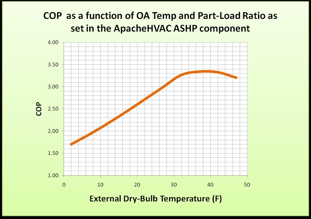
95 Figure 2-33, and VE2014 ApacheHVAC 86

96 Figure 2-34 above, the COP for the fully loaded heat pump at the 47 F rating condition would be 4.0, and this is the outdoor temperature at which the full rated capacity would be available. However, when sized to meet the full load at 32 F, the heat pump load is 81% of full load at 47 F outdoor temperature for this example. Thus the maximum COP of 3.35 occurs at an outdoor temperature of approximately 37 F and 95% load and the COP is just 3.2 at 47 F and 81% load. The inputs in the ASHP dialog could be extended to warmer temperatures if needed. Because the dialog accepts just 10 rows of data, the spacing between data points would need to be revised to accommodate this. Because the model uses linear interpolation between the data points provided, and the COP and capacity curves are both relatively flat between about 17 and 32 F for this particular data set, this would be the best region of the curve to be represented by a reduced density of data points. VE2014 ApacheHVAC 87

97 2.7 Heat Transfer Loop The heat transfer loop component is developed firstly to facilitate the simulation of water-to-air heat pump (WAHP) systems in VE 2012 (v6.5). In this first phase, the heat transfer loop must serve water-to-air heat pumps. It will eventually be extended to support heating, cooling, and collecting or rejecting heat via hot/cold-water coils on the airside network and to serve the purpose of transferring heat between other water loops (heat transfer loops, chilled water loops, hot water loops, etc.) Water-to-air heat pump systems A water-to-air heat pump system consists of multiple zone-level water-to-air heat pumps connected to a common water loop. The common water loop is used by each individual heat pump as a source for acquiring heat or sink for rejecting heat. Some of the WAHP units on the loop may be in cooling mode, while others may be in heating mode. For all WAHP units on given Heat transfer loop, this common loop simultaneously acts a resource for any WAHP in heating mode and a sink for any AWHP in cooling mode. A conventional WAHP system uses a boiler to add heat to the common loop and a cooling tower or fluid cooler to reject excess heat from the common water loop. This is also is referred to as a water-loop heat pump (WLHP) system, and the WAHP model includes a set of WLHP performance curves for this type of application. Typically, the boiler operates to maintain the minimum loop supply water temperature around 68 F (20 C), while the cooling tower or fluid cooler operates to maintain the maximum loop supply water temperature of something like 86 F (30 C). Between the maximum and minimum, the loop supply water temperature is allowed to float. A ground-water WAHP system uses an open water loop that draws water from a lake, well, or similar resource. The WAHP model includes a pre-defined set of GWHP performance curves for this type of application. The loop water temperature is assumed to float with both the loads and the lake/well water temperature, with the latter represented as an annual temperature profile on the source side of a waterto-water heat exchanger. Typical rating conditions in terms of water loop temperatures for this type of system are 50 F (10 C) for heating and 59 F (15 C) for cooling. A ground-source heat pump system uses a closed loop of polymer tubing acting as a geo-thermal heat exchanger. The loop water temperature floats with the ground temperature, loop load, and the characteristics of the geo-thermal heat exchanger. Typical rating conditions in terms of common water loop temperatures for this type of system are 32 F (0 C) for heating and 77 F (25 C) for cooling. User should be cautioned, however, that this model does not include detailed geo-thermal heat exchanger characteristics or the capacitance or thermal mass of the earth around the tubes, and therefore has no means of determining the extent to which this earth may become thermally depleted or saturated over time. So, while this model can be used to represent a ground-source heat pump system, it is limited to representing that which can be suitably described by a seasonal ground-source temperature profile. For more detailed modeling of ground-source heat pump systems, including characteristics of bore fields and geo-thermal heat exchangers, see Appendix D: Ground-Source Heat Pump Modeling using ApacheHVAC loads and Gaia Geothermal Ground-Loop Design. Two components are provided for modeling WAHP systems: Water-to-air heat pump Heat transfer loop VE2014 ApacheHVAC 88

98 The WAHP units must be connected to (served by) a common Heat Transfer Loop (HTL) by selecting the appropriate HTL within the heating/cooling coil dialogs. Details of the Water-to-air heat pump component and modeling are covered in section 2.9. This section provides details for the Heat transfer loop component. Heat sources (or sinks) available on the heat transfer loop may include the following: For heating: solar water heater (SWH), water source heat exchanger (WSHX), condenser heat recovery (CHR), air-to-water heat pump (AWHP), combined heat and power (CHP), sequenced heating equipment set For cooling: water source heat exchanger (WSHX), cooling tower (CT) or fluid cooler (FC) Note that the ground-water heat pump implementation in this phase is intended for modeling ambientand ground-water sources (oceans, rivers, lakes, ground water, wells, etc.) with a constant or readily profiled water temperature. If you choose to use this component to model a ground loop above the water table (i.e., a geo-thermal heat exchanger ), please be aware that this will not include a dynamic model of the ground mass as a source and sink to be thermally depleted and recharged over time. For more detailed modeling of ground-source heat pump systems, including characteristics of bore fields and geothermal heat exchangers, see Appendix D: Ground-Source Heat Pump Modeling using ApacheHVAC loads and Gaia Geothermal Ground-Loop Design Heat transfer loop configurations Two options are offered for the Heat transfer loop configuration: Primary-only: Loop flow is maintained by a primary pump that can be either a variable-speed pump (i.e., using a variable-speed drive) or constant-speed pump riding the pump curve. Primary-Secondary: Loop flow is maintained by a combination of primary and secondary pumps. The primary pump is assumed to have constant flow when it is on. The secondary pump can be either a variable-speed pump with VSD or a constant-speed pump riding the pump curve. Selecting the Primary only configuration effectively removes the constant-speed primary loop pump from the diagram in Figure VE2014 ApacheHVAC 89

99 Figure 2-35: Heat transfer loop with primary-secondary configuration, a range of optional heat acquisition and heat rejection devices, and zone-level water-loop (water-to-air) heat pumps. The fluid cooler alternative to the cooling tower and available heat recovery connections are not shown. Figure 2-35 shows the conceptual heat transfer loop configuration. In this configuration, the heat transfer loop uses a primary-secondary loop configuration. On the secondary loop, source water is supplied to multiple water-to-air heat pump units connected in parallel. Water-to-air heat pump units are used to serve both simple heating coils and simple cooling coils. A optional solar water heater can be included on the return side of the secondary loop, downstream of the heat pumps (i.e., as a pre-heating source on the secondary return pipe). On the primary loop, there are five optional heat sources connected in a pre-defined series configuration. These heat sources could include: WSHX (water source heat exchanger), HR (Heat recovery), AWHP (Airto-water heat pump), CHP (Combined heat and power), and sequenced boiler(s) or similar equipment in a Heating equipment set. Each of these, when included, adds heat to raise the loop water temperature to the supply water temperature set point. If the first device in line to do so does not achieve the set point, the next device in series after it will have the opportunity to address the remaining load. There are also heat rejection devices connected in series on the primary loop. These heat rejection devices can include: WSHX (water source heat exchanger) and cooling tower or fluid cooler. The water source heat exchanger, as noted above, can also function as a heat source. The modeling and dialog are VE2014 ApacheHVAC 90

100 set up to assume that the WSHX is a single device that may, if desired, operate in both heat-acquisition and heat-rejection modes. The cooling tower option comprises a separate loop with open cooling tower, water-to-water heat exchanger (WWHX), and cooling tower loop pump. The cooling tower loop is thus connected to the HTL through the WWHX, which is included to reflect the real-world need to prevent contaminants from entering the HTL. The cooling tower loop with pump and heat exchanger can alternatively be replaced with a fluid cooler, as waterside of the fluid cooler is fully contained within its integral water-to-air heat exchanger. rejecting heat to cool down the source water return temperature to source water supply temperature set point when needed Loop control and sequencing The loop water returned from each of the WAHPs served by a particular heat transfer loop (each with its own return water temperature and required flow rate) is mixed at the loop return pipe to provide the overall loop return water temperature. The loop return water temperature is then compared with the target loop supply water temperature set points to determine the loop operating mode, as the following: If any WAHP served by a particular heat transfer loop is operating (extracting heat from or rejecting heat to the HTL), the system and loop flow will be turned on. o o o If the return water temperature is lower than the loop heating supply water temperature set point, then the loop will operate in heating mode. If the return water temperature is higher than the loop cooling supply water temperature set point, then the loop will operate in cooling mode. If the return water temperature is between the loop heating and cooling supply water temperature set points, then the loop temperature will be allowed to float between these setpoints without engaging or loading any of the system-level heat acquisition or heat rejection devices. If no WAHP served by a particular heat transfer loop is currently operating, the loop, and hence the entire system, will remain off. Heating mode operation The heat acquisition sequence on a heat transfer loop, assuming all possible pre-heating devices are present, is as follows: SWH WSHXCHRAWHPCHPHeating equipment set. Unused preheating devices will be skipped in the loading sequence. When included, the sequenced Heating equipment set associated with a heat transfer loop meets remaining load after heat available from any included solar water heater (SWH), water source heat exchanger (WSHX), condenser heat recovery (CHR), air-to-water heat pump (AWHP), or combined-heat & power (CHP) system have been fully utilized. Heat available from any of these devices (SWH, WSHX, CHR, AWHP, and CHP) is thus used to meet the load prior to engaging the sequenced equipment in the Heating equipment set (see Heating equipment set sub-tab of the Heat acquisition tab in the Heat transfer loop dialog). Cooling mode operation When included, the WSHX is loaded first to meet the imposed cooling load. Any load remaining after the WSHX is met by loading the available cooling tower or fluid cooler. Note that it is possible for a WSHX on a heat transfer loop to operate in both heating and cooling modes, depending on the relative temperatures of the HTL water and WSHX source water. VE2014 ApacheHVAC 91

101 2.7.4 Loop capacity and feedback to WAHPs If the loop heating or cooling load exceeds the combined capacity of all heating equipment and heat acquisition and rejection devices available on the loop, any deficiency in overall heat transfer loop capacity will result in a deviation of the loop supply water temperature from the loop heating or cooling supply water temperature set point. HTL supply water temperature thus provides feedback to the WAHPs. In other words, while heating or cooling sources on a Heat transfer loop will always attempt to achieve the target supply water temperature, this may not be feasible under all simulated conditions. If the target supply water temperature range on the HTL cannot be maintained, the WAHPs served must attempt to meet heating or cooling loads with cooler or warmer water. The WAHPs served by the HTL will respond to the adjusted loop supply water temperature in its capacity and efficiency calculations, as the loop supply water temperature features as one of the independent variables in the WAHP performance curves Heat transfer loop sizing procedure The sizing approach used for the heat transfer loop differs from that of the chilled water and hot water loops, which always use the chiller or heating equipment set, respectively, as the primary sizing target. The sizing approach used for the HTL is to have the user nominate the Principal equipment for sizing from amongst the heating and cooling sources on the loop, and make this the focus for sizing operations. For heating, the Principal equipment for sizing may be a sequenced heating equipment set, a watersource heat exchanger, or an air-to-water heat pump; however, it may not be a solar water heater, which is not amenable to sizing by any simple procedure. The principal equipment will be sized to provide the entire loop heating load (and subject to the oversizing factor in the main HTL tab). Other devices feeding heat into the loop are sized to a specified percentage of the loop heating capacity. The Current loop capacity is the heating capacity of the principal equipment (which may have been manually edited). Cooling sizing proceeds along similar lines. Here the principal equipment may be a cooling tower with heat exchanger, fluid cooler, or water-source heat exchanger. Based on this approach, in the system-level ASHRAE Loads autosizing run (Analysis type = ApacheHVAC system loads), two design loads will be calculated for the heat transfer loop: a) Design heat acquisition load for heating b) Design heat rejection load for cooling Firstly, the design heat acquisition load for heating and design heat rejection load for cooling will be used to update the respective Autosized loop heating and cooling capacities in the HTL tab of the HTL dialog. Secondly, the two design loop loads are translated according to relative capacities set for the individual heating and cooling devices on the loop. Capacities are updated for the Principal equipment for sizing and for any other devices for which the Autosize checkbox is ticked. This can be summarized as follows: Heat acquisition load (loop heating capacity) o o 100% + oversizing factor goes to the principal heating equipment (it will be sized to meet the entire loop heating load). User specified percentage (100% + oversize factor) goes to other heat acquisition devices that are present and designated for autosizing. VE2014 ApacheHVAC 92

102 Heat rejection load (loop cooling capacity) o o 100% + oversizing factor goes to the principal cooling equipment (it will be sized to meet the entire loop heat rejection load). User specified percentage (100% + oversize factor) goes to other heat rejection devices that are present and designated for autosizing. Whether or not the capacity for an individual heating or cooling device will be updated with the autosized value depends on the status of its corresponding Autosize checkbox. If this checkbox is ticked for a device, its capacity will be updated with the autosized value. If this checkbox is not ticked for a device, its capacity will not be updated with the autosized value. In addition to the capacities for the heat transfer loop and individual heating and cooling devices, the following two design temperatures will also be updated after a system sizing run: Design outdoor dry-bulb temperature on the Heat rejection tab of the HTL dialog Design outdoor wet-bulb temperature on the Heat rejection tab of the HTL dialog Heat transfer loop pump modeling As noted above, there are two options for the Heat transfer loop configuration: Primary-only: Loop flow is maintained by a primary pump that can be either a variable-speed pump (i.e., using a variable-speed drive) or constant-speed pump riding the pump curve. Primary-Secondary: Loop flow is maintained by a combination of primary and secondary pumps. The primary pump is assumed to have constant flow when it is on. The secondary pump can be either a variable-speed pump with VSD or a constant-speed pump riding the pump curve. For both Heat transfer loop configurations, pumps are assumed to operate whenever at least one WAHP unit served by the HTL is operating i.e., whenever there is heat rejection to or heat acquisition from the HTL. Otherwise, all pumps remain off and there is no water loop flow. If the pump has a constant flow when it is on, as is true for the primary pump in the Primary-Secondary configuration, this constant flow is multiplied by its specific pump power to determine the pump power. If the pump has variable flow, which can be the case for the primary pump in the Primary-only configuration or the secondary pump in the Primary-Secondary configuration, its design pump power is calculated as the specific pump power multiplied by the design water flow rate. The design pump power is then modified by the pump power curve to get the operating pump power. If a pump has variable flow it will be subject to cycling on/off below the minimum flow rate permitted. The variable flow featured in the pump power curve is calculated as the sum of flow required from all WAHPs served by the heat transfer loop, subject to the minimum flow permitted for the pump. Required water flow rates for the WAHPs vary in proportion to their heat rejection or heat acquisition loads. When the Primary-only configuration is selected for the Heat transfer loop, this effectively removes the constant-speed primary loop pump from the diagram in Figure Heat transfer loop distribution losses and pump heat gain Distribution losses from the pipe work are considered as a user-specified percentage of the heat transfer loop load. Transfer of loop pump heat gain to the loop is modeled according to a user input fraction for pump and motor heat gain to the heat transfer loop. VE2014 ApacheHVAC 93

103 2.7.8 Heat transfer loops dialog The heat transfer loops tool provides access to adding, editing, copying, and removing named heat transfer loops. Toolbar button for Heat transfer loops. Clicking this toolbar button opens up the Heat transfer loops dialog (shown in Figure 2-36), which manages the list of heat transfer loops. A heat transfer loop may be added, edited, removed, or copied through the corresponding buttons in this dialog. Double clicking on an existing heat transfer loop, or clicking the Edit button after selection of an existing heat transfer loop, opens the Heat transfer loop dialog (shown in Figure 2-37) where parameters for the selected loop may be edited. Figure 2-36: Heat transfer loops dialog shown with illustrative default loop included with the pre-defined systems in VE 2012 (v6.5) Heat transfer loop dialog The Heat transfer loop dialog has five tabs: Heat transfer loop: This tab manages the properties of the heat transfer loop. It provides inputs for the loop principle equipment for sizing, information on loop capacity and flow, as well as inputs for the primary and secondary loop pumps. Temperature control: This tab provides inputs for the loop temperature controls. Heat acquisition: This tab manages information used for all devices available for adding heat to the loop (SWH, CHR, AWHP, CHP, and Heating equipment set), except for the WSHX, which can be used as both heating and cooling source and is presented on its own in a separate tab. Water-source heat exchanger: This tab provides inputs for the WSHX, which can be used to add heat to or reject heat from the loop. VE2014 ApacheHVAC 94

104 Heat rejection: This tab manages information used for heat rejection devices (cooling tower or fluid cooler) on the loop, except the WSHX, which can be used as both heating and cooling source and is presented on its own in a separate tab. Figure 2-37: Heat transfer loop dialog shown with the Heat transfer loop tab selected Reference name for Heat transfer loop Enter a description of the component to aid in selecting and referencing any component or controllers within other dialogs and in the component browser tree. Reference names should be informative with respect to differentiating similar equipment, components, and controllers. VE2014 ApacheHVAC 95

105 Sizing status The sizing status is an informative field indicating whether the design calculation is feasible for the current settings of all relevant heat transfer loop input parameters. The sizing status is checked and updated instantaneously in response to any changes on the parameters that the following derived parameters depend upon, provided that these derived parameters are active (enabled): a) Loop flow rate in the HTL tab b) HX design approach and design effectiveness in the WSHX tab c) Fluid cooler or cooling tower design approach in the Heat rejection tab d) Cooling tower HX design approach and design effectiveness in the Heat rejection tab For the above derived parameters to be considered as feasible: a) HTL loop flow rate should be > 0.0; b) WSHX design approach should be 0.0 K; c) WSHX design effectiveness (ɛ) should be: 0.0 ɛ 1.0; d) Fluid cooler design approach should be 0.01 K; e) Cooling tower design approach should be 0.01 K; f) Cooling tower HX design approach should be 0.0 K; g) Cooling tower HX design effectiveness (ɛ) should be: 0.0 ɛ 1.0; When an individual derived parameter is feasible, it is displayed in black text. When all of the above derived parameters are feasible, the sizing status field displays Design calculation successful. If any of the above derived parameters is infeasible (out of range), the infeasible derived parameter is displayed (on the interface) in red text, and the sizing status field displays Design calculation failed. The parameters in red are out of range. in red text Heat transfer loop tab The Heat transfer loop tab facilitates the definition of the loop principle equipment for sizing, loop capacity and flow, the primary and secondary loop pumps, together with the distribution losses and oversizing factor for the heat transfer loop Distribution Losses Enter the heat transfer loop distribution losses i.e., the loss due to distribution of heating or cooling from the heating or cooling plant to point of use as a percentage of heating or cooling demand. The loss entered here does not accrue to the conditioned spaces within the building. Rather, this heat is assumed to be lost either directly or indirectly to the outdoor environment. Warning Limits (%) 0.0 to 20.0 Error Limits (%) 0.0 to 75.0 VE2014 ApacheHVAC 96

106 Oversizing Factor Following system-level autosizing, the factor by which the heating or cooling plant equipment size is increased relative to the peak value occurring during the sizing run Principal equipment for sizing Select the principle equipment for sizing, both for heating/heat acquisition and for cooling/heat rejection. To ensure there is always at least one device available to add required heat the heat transfer loop and to reject excess heat from the loop, a principle device for heating and cooling must be selected. This selection will, in turn, force at least one device to be defined for each of these roles. There are three options for the principle heating device: Heating equipment set Water-source heat exchanger Air-to-water heat pump. There are three options for the principle cooling device: Cooling tower/fluid cooler Water-source heat exchanger Except for the case of the Override checkbox beside the Current loop capacities (see below in the loop capacity section) is ticked, the capacities of the principal devices are the basis for the Current loop capacities and loop flow rate derivation. In other words, when the Override checkbox is not ticked, the Current loop capacities (heating and cooling) are dynamic copies of the capacities of the principal devices, and these may or may not have been updated by autosizing. When the Override checkbox is ticked, the corresponding Current loop capacity becomes an input field, which allows values for Loop heating capacity or Loop cooling capacity to be overridden by a manual edit. Once overridden, the Current loop capacities, and hence the loop flow rate, are decoupled from the capacities of the principle device(s). Tip: After completing a system sizing with one principle device selected, ticking the Override checkbox and switching the principle device from the pre-sizing selection to another one provides the opportunity to turn off the pre-sizing principle device in further simulations. When a Heating equipment set is the principal heating device, capacity is given by the sum of the design heating capacities for equipment with nonzero sequencing rank in the rightmost column of the sequencing table in the Heating equipment set sub-tab of the Heat acquisition tab. Whether or not an individual heating or cooling device on the loop will be autosized after a system sizing run, regardless of principle or non-principle status for sizing, depends on the status of its Autosize checkbox (see below). If the Autosize checkbox for an individual device is ticked, its capacity will be updated after autosizing. Otherwise, its capacity will remain at the pre-sizing value. If an individual device is designated as the Principle equipment for sizing, and its Autosize checkbox is ticked, then upon autosizing the peak Heat transfer loop heating or cooling capacity determined by autosizing will be used directly to update the capacity of this individual device. In other words, a principle device with its Autosize checkbox ticked will always get 100% of the autosized loop heating or cooling capacity, after consideration of the oversizing factor. If an individual device is not the current principle device for sizing, and its Autosize checkbox is ticked, then upon autosizing the peak Heat transfer loop heating or cooling capacity determined by autosizing VE2014 ApacheHVAC 97

107 will be multiplied by its Percent of autosized loop heating or cooling capacity (see below) to determine its capacity. The resultant capacity will then be used to update the capacity of this individual device. In other words, a non-principle device with its Autosize checkbox ticked will get a percentage of the autosized loop heating or cooling capacity as specified by its Percent of autosized loop heating or cooling capacity, after consideration of the oversizing factor. In this case, the capacity fraction assigned to the non-principle device is not subtracted from the loop heating or cooling capacity. Also, for a non-principle device with its Autosize checkbox ticked, once the heat transfer loop has been sized, edits made in its Percent of autosized loop heating or cooling capacity (%) field will lead to automatic dynamic updating of its capacity, based on the autosized loop heating or cooling capacity Loop capacity and flow The Autosized loop capacities (for heating and cooling) are un-editable fields, which are initialized to zero and subsequently display the results from the most recent system auto-sizing analysis. When the Override checkbox besides the Current loop capacities is not ticked, the Current loop capacities (heating and cooling) are dynamic copies of the capacities of the principal devices (which may or may not have been updated by auto-sizing). Ticking the Override checkbox allows the Current value of the Loop heating or cooling capacity to be overridden by a manual edit (otherwise all these values are un-editable). When the Override box is ticked, after autosizing, the Current value of the associated capacity remains at the user-specified value. This value is not dynamically linked to the principle equipment sizes. Loop flow rate is derived dynamically from the Current loop capacity values, taken together with loop temperature delta-t parameters specified in the Temperature control tab. The loop flow rate feeds into dynamic parameter derivations for certain components on the loop (cooling tower, fluid cooler, watersource heat exchanger, etc.). Capacities for individual heating and cooling devices can be edited manually, overriding autosized values for the equipment. In the case of principal equipment for sizing, when the Override box is not ticked, user edits made in the principal equipment capacity will feed back to the Current value of Loop capacities. This may cause a change to Loop flow rate, which may in turn cause changes to dynamically derived parameters for other devices on the loop Loop Configuration Select the loop configuration. Two options are offered: Primary-only and Primary-Secondary Primary Circuit Specific Pump Power at Rated Speed Enter the primary circuit specific pump power at rated speed, expressed in W/(l/s) in SI units (or W/gpm in IP units). If the loop configuration is selected as Primary-only: Primary circuit pump power will be calculated on the basis of variable flow, subject to the constraint that the pump will start cycling below the minimum flow rate it permits. The operating pump power will be based on its design pump power modified by the pump power curve. Its design pump power is calculated as the specific pump power multiplied by the design water flow rate. The default value for the specific pump power in this case is the total specific pump power (19 W/gpm) as specified in ASHRAE 90.1 G VE2014 ApacheHVAC 98

108 The required variable flow featured in the pump power curve is calculated as the summation of required flow from all components (WAHPs) served by the heat transfer loop, subject to the minimum flow the pump permits. Required loop water flow rates for WAHPs vary in proportion to their heat rejection or heat acquisition loads. If the loop configuration is selected as Primary-Secondary: Primary circuit pump power will be calculated on the basis of constant flow (when it operates). The model will be based on a specific pump power parameter, with a default value of 3.8 W/gpm. The default value is based on the total specific pump power (19 W/gpm) as specified in ASHRAE 90.1 G and assuming a 20:80 split between the primary and secondary circuits. The primary circuit loop flow rate will be calculated from the Current loop capacity values, taken together with loop temperature delta-t parameters specified in the Temperature control tab Primary Circuit Pump Heat Gain to Heat Transfer Loop (fraction) Enter the primary circuit pump heat gain to heat transfer loop, which is the fraction of the motor power that ends up in the loop water. Its value is multiplied by the primary circuit pump power to get the primary circuit pump heat gain, which is added to the loop cooling load or deducted from the loop heating load Primary Circuit Pump Power Curve, f Pv (v) This field is only active when the loop configuration is selected as Primary-only. If this field is active: This is the primary circuit pump power curve currently selected. Use the Select button to select the appropriate curve from the system database. Use the Edit button to edit the curve parameters if you like. The Edit button will pop up a dialog displaying the formula and parameters of the curve, allowing the curve parameters to be edited. You are allowed to edit the curve coefficients, in addition to the applicable ranges of the curve independent variables. When editing the curve parameters, it is important that you understand the meaning of the curve and its usage in the model algorithm. Also be careful that the edited curve has reasonable applicable ranges for the independent variables. A performance curve is only valid within its applicable ranges. In the case the independent variables are out of the applicable ranges you set, the variable limits (maximum or minimum) you specified in the input will be applied. The primary circuit pump power curve f Pv (v) is a cubic function of v = V/V e where V = pump volumetric flow rate. V e = design pump volumetric flow rate. And: f Pv (v) = (C 0 + C 1 v + C 2 v 2 + C 3 v 3 ) / C norm VE2014 ApacheHVAC 99

109 where C 0, C 1, C 2 and C 3 are the curve coefficients C norm is adjusted (by the program) to make f Pv (1) = 1 The primary circuit pump power curve is evaluated for each iteration of the heat transfer loop, for each time step during the simulation. The curve value is multiplied by the design primary pump power to get the operating primary pump power of the current time step, for the current fraction of pump volumetric flow rate. The curve should have a value of 1.0 when the operating pump volumetric flow rate equals rated pump volumetric flow rate (v = 1.0). Figure 2-38: Edit dialog for the primary circuit pump power curve (values for constant-speed pump are shown) Secondary Circuit Specific Pump Power at Rated Speed This field is only active when the loop configuration is selected as Primary-Secondary. If this field is active: VE2014 ApacheHVAC 100

110 Enter the secondary circuit specific pump power at rated speed, expressed in W/(l/s) in SI units (or W/gpm in IP units). The default value (15.2 W/gpm) is based on the total specific pump power (19 W/gpm) as specified in ASHRAE 90.1 G and assuming a 20:80 split between the primary and secondary circuits. Secondary circuit pump power will be calculated on the basis of variable flow, subject to the constraint that the pump will start cycling below the minimum flow rate it permits. The operating pump power will be based on its design pump power modified by the pump power curve. Its design pump power is calculated as the specific pump power multiplied by the design loop flow rate. The design secondary circuit loop flow rate is assumed equal to the design primary circuit loop flow rate, which is calculated from the Current loop capacity values, taken together with loop temperature delta-t parameters specified in the Temperature control tab. The required variable flow featured in the pump power curve is calculated as the summation of required flow from all components (WAHPs) served by the heat transfer loop, subject to the minimum flow the pump permits. Required loop flow rates for WAHPs vary in proportion to their heat rejection or heat acquisition loads Secondary Circuit Pump Heat Gain to Heat Transfer Loop (fraction) This field is only active when the loop configuration is selected as Primary-Secondary. If this field is active: Enter the secondary circuit pump heat gain to heat transfer loop, which is the fraction of the motor power that ends up in the loop water. Its value is multiplied by the secondary circuit pump power to get the secondary circuit pump heat gain, which is added to the loop cooling load or deducted from the loop heating load Secondary Circuit Pump Power Curve, f Pv (v) This field is only active when the loop configuration is selected as Primary-Secondary. If this field is active: This is the secondary circuit pump power curve currently selected. Use the Select button to select the appropriate curve from the system database. Use the Edit button to edit the curve parameters if you like. The Edit button will pop up a dialog displaying the formula and parameters of the curve, allowing the curve parameters to be edited. You are allowed to edit the curve coefficients, in addition to the applicable ranges of the curve independent variables. When editing the curve parameters, it is important that you understand the meaning of the curve and its usage in the model algorithm. Also be careful that the edited curve has reasonable applicable ranges for the independent variables. A performance curve is only valid within its applicable ranges. In the case the independent variables are out of the applicable ranges you set, the variable limits (maximum or minimum) you specified in the input will be applied. The secondary circuit hot water pump power curve f Pv (v) is a cubic function of v = V/V e where V = pump volumetric flow rate. VE2014 ApacheHVAC 101

111 V e = design pump volumetric flow rate. and f Pv (v) = (C 0 + C 1 v + C 2 v 2 + C 3 v 3 ) / C norm where C 0, C 1, C 2 and C 3 are the curve coefficients C norm is adjusted (by the program) to make f Pv (1) = 1 The secondary circuit pump power curve is evaluated for each iteration of the heat transfer loop, for each time step during the simulation. The curve value is multiplied by the design secondary pump power to get the operating secondary pump power of the current time step, for the current fraction of pump volumetric flow rate. The curve should have a value of 1.0 when the operating pump volumetric flow rate equals rated pump volumetric flow rate (v = 1.0). Figure 2-39: Edit dialog for the secondary circuit pump power curve (values for constant-speed pump are shown) VE2014 ApacheHVAC 102

112 Temperature control tab The Temperature control tab provides inputs for the heat transfer loop temperature controls. There are two parallel sets of temperature control parameters provided in this tab: one set for heating, one set for cooling. The descriptions below for each of these temperature control parameters apply to both heating and cooling temperature controls. Figure 2-40: Temperature control tab on Heat transfer loop dialog. VE2014 ApacheHVAC 103

113 Design Loop Temperature Difference, DeltaThdes & DeltaTcdes Enter the design loop temperature difference for heating and cooling, i.e., the difference between the design loop supply water temperature and return water temperature Design Supply Water Temperature For heating, the design loop supply water temperature may be either an input field or a derived parameter (un-editable field with a grey background), depending on the currently selected heating principle equipment for sizing (in the Heat transfer loop tab). If this is an input field, enter the desired design loop supply water temperature for heating. If this is a derived parameter, then the heating design loop supply water temperature is determined by parameter inputs for the currently selected heating principle equipment for sizing, and does not need to be entered in the Temperature control tab. For cooling, the design loop supply water temperature currently is always a derived parameter (uneditable field with a grey background), and does not need to be entered in the Temperature control tab. It is determined by parameter inputs for the currently selected cooling principle equipment for sizing, which may be either Cooling tower/fluid cooler or WSHX. The default values for heating and cooling design supply water temperatures are taken as the rated WAHP entering fluid temperatures from ANSI/ARI/ASHRAE ISO Standard : Supply Water Temperature Set Point Three options are available for heating and cooling supply water temperature set point: Constant, Profiled, or Reset. Whichever option is selected, to avoid the heating and cooling set point compete each other on the loop temperature control at the same time step during a simulation, please ensure that the heating supply water temperature set point is not higher than the cooling supply water temperature set point at the same time step during a simulation. Otherwise, an error will be reported and the simulation will not be able to proceed. The software provides a check on this when it is possible, i.e., when both heating and cooling set points are specified as Constant. For all other cases, it is your responsibility to avoid the heating and cooling set point compete each other on the loop temperature control at the same time step during a simulation Constant Supply Water Temperature Set Point When Constant is selected for heating and cooling supply water temperature set point, enter the desired constant heating and cooling loop supply water temperature set point Timed Supply Water Temperature Set Point Profile When Profiled is selected for heating and cooling supply water temperature set point, select the absolute profile to be applied to the loop supply water temperature set point, which are defined through the APPro facility (the Profiles Database) Supply Water Temperature Reset Type When Reset is selected for heating and cooling supply water temperature set point, select the supply water temperature reset type. Currently only one option is provided: Outdoor air temperature reset. When Outdoor air temperature reset type is selected, which is the default, you also need to specify four more reset parameters: VE2014 ApacheHVAC 104

114 Outdoor dry-bulb temperature low limit Supply water temperature at or below low limit Outdoor dry-bulb temperature high limit Supply water temperature at or above high limit Outdoor Dry-bulb Temperature Low Limit When heating or cooling supply water temperature reset type is selected as Outdoor air temperature reset, enter the outdoor dry-bulb temperature low limit to be used by the reset Supply Water Temperature at or below Low Limit When heating or cooling supply water temperature reset type is selected as Outdoor air temperature reset, enter supply water temperature at or below the outdoor dry-bulb temperature low limit, to be used by the reset Outdoor Dry-Bulb Temperature High Limit When heating or cooling supply water temperature reset type is selected as Outdoor air temperature reset, enter the outdoor dry-bulb temperature high limit to be used by the reset Supply Water Temperature at or above High Limit When heating or cooling supply water temperature reset type is selected as Outdoor air temperature reset, enter the supply water temperature at or above the outdoor dry-bulb temperature high limit, to be used by the reset Heat acquisition tab The Heat acquisition tab manages information used for all possible heating devices (SWH, CHR, AWHP, CHP, heating equipment set) on the loop, except for the WSHX, which can be used as both heating and cooling source and is presented in its own separate tab. For each of the possible heating devices presented in this tab, there is a corresponding checkbox and an associated sub-tab. Ticking or un-ticking a checkbox will enable or disable the associated sub-tab. The hard-wired sequence for heat acquisition on a heat transfer loops is SWH WSHX CHR AWHP CHP Heating equipment set. VE2014 ApacheHVAC 105

115 Figure 2-41: Heat acquisition tab on Heat transfer loop dialog (shown with the Heating equipment set subtab selected). VE2014 ApacheHVAC 106

116 Location of Pre-heating Components Select the Location of pre-heating components on the heat transfer loop. Currently only one option is provided: Secondary return Solar water heater Solar water heater can be used as a pre-heating device on a heat transfer loop. When present, the solar water heater will be the first-loaded device to cover heating load imposed on the heat transfer loop. Solar water heater on a heat transfer loop is modeled and functions in exactly the same manner as the Solar water heater on the hot water loop (see section Solar Water Heater). Figure 2-42: Solar water heater dialog with illustrative inputs Solar water heater checkbox Tick this checkbox to specify a solar water heater as a pre-heating device on the heat transfer loop. Ticking or un-ticking this checkbox will enable or disable the associated Solar water heater sub-tab below Solar water heater reference This displays the Reference name of the solar water heater associated with this heat transfer loop. It is not editable directly in the HTL dialog and should be edited in the solar water heater dialog, which is opened by clicking the Edit button to the right of this field. VE2014 ApacheHVAC 107

117 Heat recovery Heat recovery, when enabled within the Heat transfer loop dialog, serves heat acquisition loads ahead after any solar water heating and/or water-source heat exchanger. The hard-wired sequence for heat acquisition on a heat transfer loops is SWH WSHX CHR AWHP CHP Heating equipment set. The heat recovery can be modeled as either a heat exchanger or water-to-water heat pump between loops. Most often, but not always, the recovered heat is from a condenser water loop for cooling equipment, and in that case referred to as condenser heat recovery (CHR). There are two heat exchanger and water-water heat pump (WWHP) model options for heat recovery when the recipient is a Hot water loop: a simple fixed-percentage effectiveness heat exchanger and fixed- COP heat pump or an explicit model with heat exchanger effectiveness and heat pump COP varying according to the loop water temperatures. Percentage of heat rejection heat-exchanger model This simple heat-exchanger model is essentially the same as the heat recovery model provided in pre-v6.5 versions. It models the heat recovery as a simple percentage of the source heat rejection. The percentage represents a fixed heat-exchanger effectiveness. Fixed-COP water-source heat pump model The temperature for the recovered heat can be upgraded with a water-to-water or watersource heat pump (WSHP) e.g., from 90 F to 140 F. This would typically be used when serving space-heating loads such as direct (DX-based) heating of supply air or hot water for heating coils and baseboard heaters that require higher temperatures than normally available via a simple heat exchanger on the condenser water loop. The Percentage of heat rejection model can be used regardless of whether there is an explicit modeling of the loop water temperatures on the heat recovery source and recipient sides. Explicit heat transfer: This option models the heat transfer between the heat recovery source and recipient loops using an explicit water-to-water heat exchanger, which modulates the heat exchanger effectiveness for off-design temperature differences across the heat exchanger. Variable-COP water-source heat pump model In the explicit heat transfer model, the water-to-water heat pump (WWHP) used to upgrade recovered heat modulates COP in response to the temperature difference or thermal lift between the heat recovery source loop and the heat recovery recipient loop at each simulation time step. This relatively simple model uses linear interpolation to vary the COP between two user-input COP values corresponding to two heat pump operation points (low & high thermal lift). The Explicit heat transfer model can be used only when there is an explicit modeling of the loop water temperatures on the heat recovery source and recipient sides. Capacity for the Heat Recovery WWHP is now limited to a user-specified percentage of the heat recovery source capacity, whereas in pre-v6.5 versions WWHP capacity was a percentage of the instantaneous load on the source. This revised limit has been introduced in both of the WWHP models described above in order to provide a more realistic basis for the capacity. This avoids recovering more heat with the WWHP than would be possible (or desirable) in practice. Without this constraint the WWHP could entirely displace the boilers on a HWL, which might not be what the user intends or expects. VE2014 ApacheHVAC 108

118 Heat recovery sources and recipients All heat recovery data are now displayed, edited, and stored on the recipient side (Figure 2-79 and Figure 2-17 below). Heat recovery sources can be either a part-load-curve chiller model (which may represent something other than a water-cooled chiller) or a condenser water loop serving one or more electric water-cooled chillers. Future versions will expand on the range of possible sources, for example, allowing the heattransfer loop to be selected as a source. Heat recovery recipients can be a generic heat source, a hot water loop, or a heat transfer loop. When the Percentage of heat rejection model is used, there can be multiple heat recovery sources linked to one recipient. This is among the reasons that the sources are now specified in the recipient dialog. Source types can be any combination of condenser water loops and/or part-load curve chiller models. Each heat recovery source can be linked to just one heat recipient. When the Explicit heat transfer model is used, there can be only one heat recovery source linked to a given recipient loop, and the source type is limited to condenser water loops. The heat recovery recipient is displayed on the source side (Heat recovery sub-tab within the Heat Rejection tab of the Chilled water loop dialog and in the Part-load curve chiller model dialog) for user s information only. Each heat recovery source can be linked to only one heat recovery recipient. VE2014 ApacheHVAC 109

119 Figure 2-43: Heat Recovery sub-tab on the Heat acquisition tab within the Heat transfer loop dialog (top) using the Percentage of heat rejection model with water-to-water heat pump and illustrative inputs for source, percentage heat recovery, and WWHP performance. Also shown (below the Hot water loop dialog), the Condenser heat recovery recipient designation is displayed within the Heat rejection tab of the Chilled water loop dialog. VE2014 ApacheHVAC 110

120 Figure 2-44: Heat Recovery tab within the Heat transfer loop dialog (top) using the Explicit heat transfer model with water-to-water heat pump and illustrative inputs for source, heat exchanger effectiveness, and WWHP performance. Also shown (below the Hot water loop dialog), the Condenser heat recovery recipient designation is displayed within the Heat rejection tab of the Chilled water loop dialog. VE2014 ApacheHVAC 111

121 Heat recovery checkbox Tick this checkbox to specify heat recovery as a heat source on the heat transfer loop. Ticking or un-ticking this checkbox will enable or disable the associated heat recovery sub-tab below Heat recovery model Choose the desired heat recovery model type. Two model types are provided: Percentage of heat rejection and Explicit heat transfer. If Percentage of heat rejection is selected, you will be able to specify multiple heat recovery sources contributing to the same hot water loop (the heat recovery recipient), listed in a source table below, together with other parameters required by the Percentage of heat rejection model. For each heat recovery source row in the table, these column fields are displayed: Source type, Source, Max. heat recovery with HX (%, as percentage of source loop load), Heat pump capacity (%, as percentage of source loop capacity), Heat pump COP, and Heat pump fuel. In this case, a heat recovery source can be added or removed using the Add or Delete button below the source table. Double clicking any active cell within the source table provides editing access to that specific cell. If Explicit heat transfer is selected, you will be able to specify only one heat recovery source contributing to the hot water loop (the heat recovery recipient), together with other parameters required by the Explicit heat transfer model Water-to-water heat pump checkbox The heat recovered from the heat recovery source(s) may be upgraded using a water-to-water heat pump (See additional explanation above). Specify this mode of operation by ticking the Water-to-water heat pump checkbox Source type Choose the heat recovery source type for a particular source. For the Percentage of heat rejection model, Source type is listed in the first column of the source table. Double clicking a cell in this column allows you to choose the source type from two options: Condenser water loop or Part load chiller. For the Explicit heat transfer model, Source type is selected from the Source type combo box, currently with one available option: Condenser water loop. When source type is Condenser water loop, this is referring to a condenser water loop associated with a currently defined chilled water loop. When source type is Part load chiller, this is referring to any currently defined part load chiller either on a chilled water loop or separately defined as a Generic cooling source Source Choose the heat recovery source name for a particular source. For the Percentage of heat rejection model, Source is listed in the second column of the source table. Double clicking a cell in this column allows you to choose the source from a drop-down list of available sources currently defined in the HVAC system file. For the Explicit heat transfer model, use the Source drop-down list on the right hand side of the dialog to select from available sources currently defined in the HVAC system file. VE2014 ApacheHVAC 112

122 Note that for both heat recovery models, only the current available sources defined in the HVAC file will be included in the drop-down list: If the selected Source type is Condenser water loop, available means the listed chilled water loop has a condenser water loop (Condenser water loop box on Heat rejection tab is ticked) that has not been specified as a heat recovery source for any other heat recovery recipient. If the selected Source type is Part-load chiller, available means the defined part-load chiller has not been specified a heat recovery source for any other heat recovery recipient. On switching the model option from Percentage of heat rejection to Explicit heat transfer, no more than one source will remain active and displayed (and this must not be a part load curve chiller). If there are multiple sources specified prior to the switch and these include more than one valid source for the Explicit heat transfer option, then the first valid source for the Explicit heat transfer option will remain; other specified sources will be removed. If prior to the switch, there are only part load curve chillers specified as sources, then upon switching the Source combo list will be set to <None>. For a specified heat recovery source, its recipient will be displayed in the corresponding source dialog for user s information only Max. heat recovery with HX (%) This parameter is only required by the Percentage of heat rejection model. When Percentage of heat rejection model is used, this field (in the 3 rd column of the source table) represents the percentage of the source heat rejection (from either a condenser water loop or a part load chiller) that is subject to heat recovery using a heat exchanger. In this case, the amount of heat recovered at any given time is given by: ( Ql Heat Recovered Qc ) p 100 Where, Q l is the load on the electric water-cooled chiller(s) if the heat recovery source is a condenser water loop (or the load on the part load curve chiller if the source is from a part load chiller), Q c is the compressor power for the chiller(s) and p is heat recovery percentage Heat exchanger design effectiveness This parameter is only required by the Explicit heat transfer model. When Explicit heat transfer model is used, it represents the design effectiveness of the water-to-water heat exchanger used for heat recovery purpose Heat pump capacity (%) This field is only enabled when the Water-to-water heat pump checkbox is ticked, i.e., when a water-towater heat pump is used to upgrade the heat recovered from the source(s). When active, enter the capacity for the desired water-to-water heat pump, as a percentage of the source loop capacity. This is used to limit the capacity of the water-to-water heat pump. When heat recovery source is a condenser water loop: the source loop capacity is the cooling tower or fluid cooler capacity (the condenser water loop capacity). When heat recovery source is a part load chiller: the source loop capacity is the part load chiller heat rejection capacity. For the Percentage of heat rejection model, heat pump capacity is listed in the 4 th column of the source table. Double clicking a cell in this column allows you to manually edit its value. VE2014 ApacheHVAC 113

123 For the Explicit heat transfer model, heat pump capacity can be edited in the named field Heat pump COP This field is only enabled when the Water-to-water heat pump checkbox is ticked, i.e., when a water-towater heat pump is used to upgrade the heat recovered from the source(s). When active, enter the COP(s) for the desired water-to-water heat pump. For the Percentage of heat rejection model, heat pump COP is listed in the 5 th column of the source table. Double clicking a cell in this column allows you to manually edit its value, which should normally be the COP for this equipment when the source loop and recipient loop are at design temperatures; however, this may differ for some system designs. In this case, the specified COP is applied as a constant for a WWHP coupled to a specific heat recovery source during simulation. For the Explicit heat transfer model, heat pump COP can be edited in the named field at two operating points corresponding to the two Heat pump thermal lifts (two delta-t data points) that you could specify (see below). In this case, instead of using a constant COP for the WWHP, the WWHP COP will be made responsive to the thermal lift between the heat recovery source loop and the heat recovery recipient loop during the simulation: linear interpolation will be applied to 1/COP using the two heat pump COP values corresponding to the two specified operation points (low, high) Heat pump thermal lift (two delta-t data points) This field is only required by the Explicit heat transfer model, and is only enabled when the Water-towater heat pump checkbox is ticked, i.e., when a water-to-water heat pump is used to upgrade the heat recovered from the source(s). When active, enter the two heat pump thermal lifts (two delta-t data points: low, high) for the desired water-to-water heat pump. The thermal lift of the WWHP is the difference between the heat recovery source-side loop temperature before heat pump heat recovery and the recipient-side loop water temperature after heat recovery (which will ideally be the target supply water temperature of the recipient loop). During simulation, linear interpolation will be applied to 1/COP using the two heat pump COP values (see above) corresponding to the two specified thermal lifts (low, high) Heat pump fuel This field is only enabled when the Water-to-water heat pump checkbox is ticked, i.e., when a water-towater heat pump is used to upgrade the heat recovered from the source(s). When active, select the fuel, type of energy source, or energy end-use category for the water-to-water heat pump. For scratch-built systems, this will normally be Electricity and for pre-defined systems this is set to Heating (electricity), which is an end-use designation for the ASHRAE 90.1 Performance Rating Method reports. For the Percentage of heat rejection model, heat pump fuel is listed in the last column of the source table. Double clicking a cell in this column allows you to choose the heat pump fuel for the desired water-towater heat pump coupled to a specific heat recovery source. For the Explicit heat transfer model, heat pump fuel can be selected through the named field Air-to-water heat pump An Air-to-water heat pump (AWHP) can be used as a heating device on the heat transfer loop. When present, the Air-to-water heat pump will be the first in line to meet loop heating load. The following loading sequence is pre-set for all heat transfer loops: SWH WSHX CHR AWHP CHP Heating equipment set. VE2014 ApacheHVAC 114

124 Figure 2-45: Heat acquisition tab on Heat transfer loop dialog (shown with the Air-to-water heat pump sub-tab selected) Air-to-water heat pump checkbox Tick this checkbox to specify an Air-to-water heat pump as a heating device on the heat transfer loop. Ticking or un-ticking this checkbox will enable or disable the associated Air-to-water heat pump sub-tab below. If the Air-to-water heat pump is selected as the heating principal equipment for sizing, this checkbox is automatically ticked and is not allowed to be un-ticked. The input parameters for Air-to-water heat pumps are described in section VE2014 ApacheHVAC 115

125 Air-to-water heat pump reference This displays the reference name of the Air-to-water heat pump associated with this heat transfer loop. It is not editable directly in the HTL dialog and should be edited in the Air-to-water heat pump dialog, which is opened by clicking the Edit button to the right of this field. The input parameters for Air-to-water heat pumps are described in section The Edit button opens the Air-to-water heat pump dialog. Figure 2-46: Air-to-water heat pump dialog with illustrative inputs (described in section 2.6.2) Autosize air-to-water heat pump Tick this checkbox to autosize the associated Air-to-water heat pump during a system sizing run. When this box is ticked: If the air-to-water heat pump is selected as the heating principal equipment for sizing, then the peak Heat transfer loop heating capacity determined by autosizing will be used directly to update the part-load capacity (output) values in the Air-to-water heat pump dialog. In other words, the heat pump will get 100% of the autosized loop heating capacity, after consideration of the oversizing factor. If the air-to-water heat pump is not selected as the heating principal equipment for sizing, then the peak Heat transfer loop heating capacity determined by autosizing will be multiplied by the Percent of autosized loop heating capacity (%) (see below) to determine the Air-to-water heat pump capacity. The resultant maximum heat pump capacity value will then be used to update the part-load capacity (output) values in the Air-to-water heat pump dialog. In other words, the heat pump will get a percentage of the autosized loop heating capacity as specified by its Percent of autosized loop heating capacity (%), after consideration of the oversizing factor. Note that in this case, the capacity fraction assigned to the heat VE2014 ApacheHVAC 116

126 pump is not subtracted from the heat transfer loop heating capacity. In other words, the air-to-water heat pump size will not influence the size of the heat transfer loop. The capacity updating process for an Air-to-water heat pump after autosizing will reset the capacity (output) value in the bottom row and proportionally adjust all other part-load capacity values to maintain their relationships as load fractions Percent of autosized loop heating capacity (%) This field is only enabled when the air-to-water heat pump is not selected as the current heating principal equipment for sizing and its Autosize air-to-water heat pump checkbox (see above) is ticked. When this field is enabled, during a system sizing run, the autosized loop heating capacity will be multiplied by the value in this field to get the heat pump capacity. The resultant heat pump capacity will then be used to update the air-to-water heat pump capacity in the normal way (re-set the value in the bottom row and adjust all other to maintain proportional relationships in the heat pump data lines). Once the heat transfer loop has been sized, edits made in this field will lead to automatic dynamic updating of the heat pump capacity and adjusting of all other data lines in the associated heat pump dialog, based on the autosized loop heating capacity. Note that the capacity fraction assigned to the heat pump is not subtracted from the loop heating capacity. In other words, the Air-to-water heat pump size will not influence the Heat transfer loop sizing Combined heat and power Heat available from a Combined heat and power (CHP) system can be used as a heat source on the heat transfer loop. When present, heat available from the CHP system will be used to cover loop heating load prior to engaging the Heating equipment set on the Heat transfer loop, according to the following loading sequence: SWHWSHXCHRAWHPCHPHeating equipment set. A CHP system is defined within the CHP section of the Renewables dialog in the Apache Thermal view. VE2014 ApacheHVAC 117

127 Figure 2-47: Heat acquisition tab on Heat transfer loop dialog (shown with the CHP sub-tab selected) Combined heat and power checkbox Tick this checkbox to specify Combined heat and power (CHP) system as a heat source on the heat transfer loop. Ticking or un-ticking this checkbox will enable or disable the associated CHP sub-tab below CHP sequence ranking CHP sequence ranking determines the sequence in which heat available from CHP are used to cover heating loads imposed on the specified heat sources. Heat sources (Generic, Hot water loop, or Heat transfer loop) with lower values of this parameter will receive available heat from CHP before those with higher values. The former will normally be the most efficient heat sources. If two ApacheHVAC heat sources have the same sequence ranking in this field, they will simultaneously receive available heat from the CHP system in Apache Thermal until either the loads are met or the CHP resource is fully utilized Heating Equipment Set A Heating equipment set can be used as heat source on the heat transfer loop. When present, the Heating equipment set will be the last in line to meet loop heating load. The following loading sequence is pre-set for all heat transfer loops: SWHWSHXCHRAWHPCHPHeating equipment set. The Heating equipment set sub-tab, which is enabled by ticking the Heating equipment set checkbox, facilitates the definition of the heating equipment serving the heat transfer loop. Heating equipment can be added, edited, copied and removed from the existing heating equipment list (the first column of the VE2014 ApacheHVAC 118

128 sequencing table). Heating equipment can also be imported from an existing heat transfer loop using the Import button. A heating equipment sequencing table is provided to set the order in which heating equipment are turned on within any particular load range and to set the relative weighting of autosized capacities. Tick boxes are provided to activate up to 5 load ranges for sequencing and the cells with white background can be edited by double clicking. The cells containing heating equipment names in the heating equipment list column provide access to editing individual heating equipment. Figure 2-48: Heat acquisition tab on Heat transfer loop dialog (shown with the Heating equipment set sub-tab selected). VE2014 ApacheHVAC 119

129 Heating equipment set checkbox Tick this checkbox to specify Heating equipment set as a heat source on the heat transfer loop. Ticking or un-ticking this checkbox will enable or disable the associated Heating equipment set sub-tab below. If the Heating equipment set is selected as the heating principal equipment for sizing, this checkbox is automatically ticked and is not allowed to be un-ticked Autosize heating equipment set Tick this checkbox to autosize the associated Heating equipment set during a system sizing run. When this box is ticked: If the Heating equipment set is selected as the heating principal equipment for sizing, then the peak Heat transfer loop heating capacity determined by autosizing will be used directly to update the capacity of the Heating equipment set. In other words, the Heating equipment set will get 100% of the autosized loop heating capacity, after consideration of the oversizing factor. If the Heating equipment set is not selected as the heating principal equipment for sizing, then the peak Heat transfer loop heating capacity determined by autosizing will be multiplied by the Percent of autosized loop heating capacity (%) (see below) to determine and update the Heating equipment set capacity. In other words, the Heating equipment set will get a percentage of the autosized loop heating capacity as specified by its Percent of autosized loop heating capacity (%), after consideration of the oversizing factor. Note that in this case, the capacity fraction assigned to the Heating equipment set is not subtracted from the heat transfer loop heating capacity. In other words, the Heating equipment set size will not influence the size of the heat transfer loop. The resultant Heating equipment set capacity value (from either of the above two cases) will then be used to update the capacities of individual heating equipment defined for the Heating equipment set. The capacities of individual heating equipment are derived by distributing the Heating equipment set capacity using capacity weightings specified for individual heating equipment Percent of autosized loop heating capacity (%) This field is only enabled when the Heating equipment set is not selected as the current heating principal equipment for sizing and its Autosize heating equipment set checkbox (see above) is ticked. When this field is enabled, during a system sizing run, the autosized loop heating capacity will be multiplied by the value in this field to get the Heating equipment set capacity. The resultant Heating equipment set capacity will then be used to update the capacities of individual heating equipment defined for the Heating equipment set in the normal way (distributing the Heating equipment set capacity using capacity weightings specified for individual heating equipment). Once the heat transfer loop has been sized, edits made in this field will lead to automatic dynamic updating of the Heating equipment set capacity and adjusting of capacities for individual heating equipment associated with this Heating equipment set, based on the autosized loop heating capacity. Note that the capacity fraction assigned to the Heating equipment set is not subtracted from the loop heating capacity. In other words, the Heating equipment set size will not influence the Heat transfer loop sizing Heating Equipment Model Type to Add This selection determines the type of heating equipment model to be added when clicking the Add button. Currently two model types are available: part load curve heating plant and hot water boiler. VE2014 ApacheHVAC 120

130 The Heating equipment set can include any combination of two different heating equipment types: Hot water boiler: uses editable pre-defined curves and other standard inputs, such as efficiency at rated condition, supply temperature, flow rate, and parasitic loads Part load curve heating plant: flexible generic inputs entered in a matrix of load-dependent efficiency and parasitic power i.e., a data grid with efficiency and pump/parasitic power set relative to maximum and part-load values; can represent any device used to heat water Heating equipment List The heating equipment list column lists the heating equipment in the Heating equipment set for the current Heat transfer loop. Up to 10 separate pieces of heating equipment can be listed and sequenced. To open the Edit dialog for any particular heating equipment, double-click a heating equipment name on the list or select a heating equipment item and click the Edit button Heating equipment Type The heating equipment type column indicates the model type for each piece of equipment on the list. The types are determined when the heating equipment is added. PLE = Part-load equipment HWB = Hot-water boiler Part Load Range (up to %) The part load range (%) values can be edited, with the exception of the last value (100%). Up to five partload ranges can be set. Apart from unused columns those with no check in the box at the bottom of the column, and thus grayed-out values part load range values must always increase from left to right Heating equipment Sequence Rank Heating equipment sequence ranks are entered in the body of the table, for each heating equipment and for each part load range. These are integers in the range of 0 to 99 that determine the order in which heating equipment will be engaged during simulation. Within a specific part load range, heating equipment with lower sequence rank will be engaged first. At least one piece of heating equipment should have a nonzero sequencing rank in every column. When multiple heating equipment are specified to have the same sequence rank for a part load range, they will be engaged simultaneously within that part load range and will share the loop load in proportion to their design capacities. Within any range (except the last), if all the specified heating equipment are operating at maximum output, the sequencing moves to the next range. Note: If the loop heating load exceeds the combined capacity of all heating sources available on the loop, any deficiency in overall heat transfer loop capacity will result in a deviation of the loop supply water temperature from the loop heating supply water temperature set point, thus providing feedback to the WAHPs served by the heat transfer loop. In other words, heating sources on a Heat transfer loop will always attempt to achieve the target supply water temperature. If the target supply water temperature cannot be reached, the WAHPs served must attempt to meet heating loads with cooler water. The WAHPs served by the HTL will respond to the adjusted loop supply water temperature in its capacity and efficiency calculations, as the loop supply water temperature features as one of the independent variables in the WAHP performance curves. VE2014 ApacheHVAC 121

131 Heating Equipment Autosizing Capacity Weighting Heating equipment autosizing capacity weighting is a column of values indicating the relative proportion of the load that each piece of heating equipment will take during autosizing. If the rightmost sequence rank is zero for any heating equipment, the corresponding autosizing capacity weighting will be set automatically to zero. Any heating equipment with a zero autosizing capacity weighting will not be autosized. The Distribute as % button normalizes the autosizing capacity weightings so that they sum to 100. When all the autosizing weightings are zero the Distribute as % button is disabled. It is not obligatory to use the Distribute as % button, as the values will be normalized automatically when applied Active Sequence Columns Under each part load range column of the heating equipment sequencing table (except the 100% column), there is a checkbox indicating the current status of the column. These checkboxes can be ticked only from right to left and un-ticked only from left to right. When a check box is ticked, it will populate the column immediately above it with the data from the column to the right of it, thereby rendering the column immediately above it editable. The next checkbox for column immediately to the left of this checkbox will be enabled as well Water-source heat exchanger tab The Water-source heat exchanger tab provides inputs for the water-source heat exchanger, which can be used as both heating and cooling source of the loop. When present, the water-source heat exchanger will be first in line to cover heating or cooling load imposed on the heat transfer loop, following the preset loading sequence for heating or cooling: Heating: SWHWSHXCHRAWHPCHPHeating equipment set Cooling: WSHXCooling tower (or fluid cooler) In addition to the source water parameters (in the Source water section), there are two sets of design parameters required for the water-source heat exchanger (in the Water-to-water heat exchanger design parameters section): one for heating and one for cooling. Possible application for the water-source heat exchanger on the heat transfer loop is to connect it to an open water loop that draws water from a lake or well so that a ground-water system can be set up to serve WAHPs on the loop. Alternatively, the water-source heat exchanger can be connected to a closed loop utilizing a loop of plastic pipe that acts as a geo-thermal heat exchanger. However, please be reminded that the ground source implementation in this phase is restricted to ambient water sources (wells, ground water sources, rivers, lakes, etc) with a constant or profiled source water temperature. If you choose to use this component to model a ground loop above the water table (a geo-thermal heat exchanger ) please be aware of the degree of compromise involved. VE2014 ApacheHVAC 122

132 Figure 2-49: Water-source heat exchanger tab on Heat transfer loop dialog Water-source heat exchanger checkbox Tick this checkbox to specify a water-source heat exchanger as a heating and/or cooling source on the heat transfer loop. Ticking or un-ticking this checkbox will enable or disable the required water-source heat exchanger parameters below. If the water-source heat exchanger is selected as the heating or cooling principal equipment for sizing, this checkbox is automatically ticked and is not allowed to be un-ticked. VE2014 ApacheHVAC 123

133 Autosize water-source heat exchanger Tick this checkbox to autosize the water-source heat exchanger during a system sizing run. When this box is ticked: If the water-source heat exchanger is selected as the heating or cooling principal equipment for sizing, then the peak Heat transfer loop heating or cooling capacity determined by autosizing will be used directly to update the heating or cooling capacity of the water-source heat exchanger. In other words, the water-source heat exchanger will get 100% of the autosized loop heating or cooling capacity, after consideration of the oversizing factor. If the water-source heat exchanger is not selected as the heating or cooling principal equipment for sizing, then the peak Heat transfer loop heating or cooling capacity determined by autosizing will be multiplied by the Percent of autosized loop capacity (%) (see below) to determine and update the water-source heat exchanger heating or cooling capacity. In other words, the water-source heat exchanger will get a percentage of the autosized loop heating or cooling capacity as specified by its Percent of autosized loop capacity (%), after consideration of the oversizing factor. Note that in this case, the capacity fraction assigned to the water-source heat exchanger is not subtracted from the heat transfer loop heating or cooling capacity. In other words, the water-source heat exchanger size will not influence the size of the heat transfer loop Percent of autosized loop capacity (%) This field is only enabled when the water-source heat exchanger is not selected as the current heating or cooling principal equipment for sizing and its Autosize water-source heat exchanger checkbox (see above) is ticked. When this field is enabled, during a system sizing run, the autosized loop heating or cooling capacity will be multiplied by the value in this field to get the water-source heat exchanger capacity. The resultant capacity will then be used to update the water-source heat exchanger capacity. Once the heat transfer loop has been sized, edits made in this field will lead to automatic dynamic updating of the water-source heat exchanger capacity, based on the autosized loop heating or cooling capacity. Note that the capacity fraction assigned to the water-source heat exchanger is not subtracted from the loop heating or cooling capacity. In other words, the water-source heat exchanger size will not influence the Heat transfer loop sizing Source water temperature Two options are available for the water-source heat exchanger source water temperature: Constant or Profiled. When Source water temperature is selected as Constant (which is the default), the Design source-side entering temperature (for both heating and cooling) in the Water-to-water heat exchanger design parameters section will be dynamic copies of the Constant source water temperature specified in the Source water section. In this case, the Design source-side entering temperature is derived parameter and hence not editable. When Source water temperature is selected as Profiled, the Design source-side entering temperature (for both heating and cooling) in the Water-to-water heat exchanger design parameters section is input parameter and hence editable. In this case, as it is hard to automatically ensure the two design sourceside entering temperature values fall within the range set by the source water temperature profile, it will VE2014 ApacheHVAC 124

134 be your responsibility to ensure the two design source-side entering temperatures are available from the temperature profile you defined for the source water Constant source water temperature When Constant is selected for Source water temperature, enter the available constant source water temperature. In this case, the Design source-side entering temperature (for both heating and cooling) in the Water-to-water heat exchanger design parameters section will be dynamic copies of the specified Constant source water temperature Source water temperature profile When Profiled is selected for Source water temperature, select the absolute profile to be applied to the water-source heat exchanger source water temperature, which is defined through the APPro facility (the Profiles Database) Specific source water pump power Enter the specific pump power for the water-source heat exchanger source water pump, expressed in W/(l/s) in SI units (or W/gpm in IP units) Heating and Cooling radio button As the water-source heat exchanger can be used as both heating and cooling source of the heat transfer loop, there are two sets of design parameters required for the water-source heat exchanger: one for heating and one for cooling. When the Heating radio button is ticked, the heat exchanger design effectiveness derivation is based on the heat transfer coefficients derived from the heating design conditions. Also, the cooling design Approach is made a dynamic copy of the specified heating design Approach. Similarly, when the Cooling radio button is ticked, the heat exchanger design effectiveness derivation is based on the heat transfer coefficients derived from the cooling design conditions. Also, the heating design Approach is made a dynamic copy of the specified cooling design Approach Capacity Enter the heating and cooling capacities for the water-source heat exchanger. This parameter is autosizable. When this parameter is autosized, its value in the field and its autosizing label A becomes green Load-side flow rate Load-side flow rate for the water-source heat exchanger is always a dynamic copy of the Loop flow rate from the Heat transfer loop tab. It is automatically derived by the software and does not need to be specified Load-side delta T Load-side delta T for the water-source heat exchanger is the temperature difference between the heat exchanger load-side leaving temperature and load-side entering temperature. It is automatically derived by the software and does not need to be specified. VE2014 ApacheHVAC 125

135 Load-side leaving temperature Load-side leaving temperature for the water-source heat exchanger is automatically derived by the software and does not need to be specified. When the water-source heat exchanger is selected as the current heating principal equipment for sizing, the heating Design supply water temperature in the Temperature control tab will be a dynamic copy of the heating Design load-side leaving temperature in this tab. Similarly, when the water-source heat exchanger is selected as the current cooling principal equipment for sizing, the cooling Design supply water temperature in the Temperature control tab will be a dynamic copy of the cooling Design load-side leaving temperature in this tab Source-side entering temperature When Source water temperature is selected as Constant (which is the default), the Design source-side entering temperature (for both heating and cooling) in the Water-to-water heat exchanger design parameters section will be dynamic copies of the Constant source water temperature specified in the Source water section. In this case, the Design source-side entering temperature is derived parameter and hence not editable. When Source water temperature is selected as Profiled, the Design source-side entering temperature (for both heating and cooling) in the Water-to-water heat exchanger design parameters section is input parameter and hence editable. In this case, as it is hard to automatically ensure the two design sourceside entering temperature values fall within the range set by the source water temperature profile, it will be your responsibility to ensure the two design source-side entering temperatures are available from the temperature profile you defined for the source water Approach Design approach of a water-to-water heat exchanger is defined as the absolute temperature difference between its load-side leaving temperature and source-side entering temperature. When the Heating radio button (see above) is ticked, enter the heating design Approach. The cooling design Approach is made a dynamic copy of the specified heating design Approach in this case. Similarly, when the Cooling radio button (see above) is ticked, enter the cooling design Approach. The heating design Approach is made a dynamic copy of the specified cooling design Approach in this case Heat exchanger effectiveness Heat exchanger effectiveness (for heating and cooling) is automatically derived by the software using other parameters specified for the water-source heat exchanger and does not need to be specified. Note that feasible heat exchanger effectiveness (ɛ) should be: 0.0 ɛ 1.0. When the heat exchanger design effectiveness derived using the specified heat exchanger parameters is out of the feasible range, the Sizing status at the top of the Heat transfer loop dialog will report an error message in red text and a mouse-over tip over the out-of-range effectiveness (shown as red value in the field) will be given to adjust the heat exchanger parameters so that a feasible effectiveness can be derived Source-side delta T Source-side delta T for the water-source heat exchanger is the temperature difference between the heat exchanger source-side leaving temperature and source-side entering temperature. VE2014 ApacheHVAC 126

136 Given the heat exchanger capacity, the calculation of the Source-side delta T and the Source-side flow rate (see below) is interchangeable. You can choose to either enter the Source-side delta T or the Source-side flow rate and the software will automatically derive the other. The [ symbol besides the Source-side delta T and the Source-side flow rate fields indicates this interchangeable relation Source-side flow rate Given the heat exchanger capacity, the calculation of the Source-side delta T (see above) and the Sourceside flow rate is interchangeable. You can choose to either enter the Source-side delta T or the Sourceside flow rate and the software will automatically derive the other. The [ symbol besides the Source-side delta T and the Source-side flow rate fields indicates this interchangeable relation Heat rejection tab The Heat rejection tab manages information used for cooling devices (cooling tower or fluid cooler) on the heat transfer loop, except the WSHX, which can be used as both heating and cooling source and is presented in its own separate tab (see above). VE2014 ApacheHVAC 127

137 Figure 2-50: Heat rejection tab on Heat transfer loop dialog (shown with the Cooling tower with heat exchanger sub-tab selected) Design Outdoor Dry-bulb Temperature Enter the design outdoor dry-bulb temperature. This parameter is autosizable. When this parameter is autosized, its value in the field and its autosizing label A become green. VE2014 ApacheHVAC 128

138 Design Outdoor Wet-bulb Temperature Enter the design outdoor wet-bulb temperature. This parameter is autosizable. When this parameter is autosized, its value in the field and its autosizing label A become green Cooling tower or fluid cooler checkbox Tick this checkbox to specify either a cooling tower or a fluid cooler as a cooling source on the heat transfer loop. Ticking or un-ticking this checkbox will enable or disable the required cooling tower or fluid cooler parameters below. If the cooling tower or fluid cooler is selected as the cooling principal equipment for sizing, this checkbox is automatically ticked and is not allowed to be un-ticked Autosize heat rejection device Tick this checkbox to autosize the heat rejction device (cooling tower or fluid cooler) during a system sizing run. When this box is ticked: If the cooling tower or fluid cooler is selected as the cooling principal equipment for sizing, then the peak Heat transfer loop cooling capacity determined by autosizing will be used directly to update the cooling capacity of the cooling tower or fluid cooler. In other words, the cooling tower or fluid cooler will get 100% of the autosized loop cooling capacity, after consideration of the oversizing factor. If the cooling tower or fluid cooler is not selected as the cooling principal equipment for sizing, then the peak Heat transfer loop cooling capacity determined by autosizing will be multiplied by the Percent of autosized loop cooling capacity (%) (see below) to determine and update the cooling tower or fluid cooler cooling capacity. In other words, the cooling tower or fluid cooler will get a percentage of the autosized loop cooling capacity as specified by its Percent of autosized loop cooling capacity (%), after consideration of the oversizing factor. Note that in this case, the capacity fraction assigned to the cooling tower or fluid cooler is not subtracted from the heat transfer loop cooling capacity. In other words, the cooling tower or fluid cooler size will not influence the size of the heat transfer loop. Note that in both cases, if the heat rejection device is cooling tower with heat exchanger, the autosized loop cooling capacity or the capacity derived from the autosized loop cooling capacity is used to update the capacity of the heat exchanger, which connects the cooling tower loop to the heat transfer loop. The final cooling tower capacity will be the updated heat exchanger capacity plus the cooling tower loop pump heat gain Percent of autosized loop cooling capacity (%) This field is only enabled when the cooling tower or fluid cooler is not selected as the current cooling principal equipment for sizing and the Autosize heat rejection device checkbox (see above) is ticked. When this field is enabled, during a system sizing run, the autosized loop cooling capacity will be multiplied by the value in this field to get the cooling tower or fluid cooler capacity. The resultant capacity will then be used to update the cooling tower or fluid cooler capacity. Once the heat transfer loop has been sized, edits made in this field will lead to automatic dynamic updating of the cooling tower or fluid cooler capacity, based on the autosized loop cooling capacity. VE2014 ApacheHVAC 129

139 Note that the capacity fraction assigned to the cooling tower or fluid cooler is not subtracted from the loop cooling capacity. In other words, the cooling tower or fluid cooler size will not influence the Heat transfer loop sizing Heat rejection device When this field is active, select the heat rejection device from the available options. Presently, two options are provided: an open cooling tower with heat exchanger or a closed-circuit fluid cooler. The open cooling tower model is based on the Merkel theory, which is same as those used for the cooling tower in a chilled water loop or in a dedicated waterside economizer (see that section of the User Guide for details). The fluid cooler can be either wet, dry, or switch from wet to dry operation when outdoor temperature drops below a set threshold. For both the Cooling tower with heat exchanger and the Fluid cooler option, there is an associated sub-tab containing the parameters required by each option, which becomes active when that option is selected. The parameters associated with the Cooling tower with heat exchanger option are described immediately below. The parameters associated with the Fluid cooler option are described following the cooling tower parameters Cooling tower with heat exchanger Cooling tower is one of the optional heat rejection devices on the heat transfer loop. When present, the cooling tower will be the last-loaded device to cover cooling load imposed on the heat transfer loop, following the preset loading sequence for cooling: WSHXCooling tower (or fluid cooler). The Cooling tower with heat exchanger sub-tab becomes active when heat rejection device is selected as Cooling tower with heat exchanger. It contains design parameters for the cooling tower, the cooling tower loop pump, and the water-to-water heat exchanger connecting the cooling tower loop to the heat transfer loop Cooling tower Cooling capacity, Qhrdes Enter the cooling capacity for the cooling tower. This is the heat rejection load on the cooling tower at design condition, which needs to cover the heat rejection load imposed on the heat transfer loop and the cooling tower loop pump heat gain. This parameter is autosizable. When this parameter is autosized, its value in the field and its autosizing label A become green Loop supply temperature Loop supply temperature here is the load-side leaving water temperature for the water-to-water heat exchanger that connects the cooling tower loop to the heat transfer loop. It is automatically derived by the software using other specified parameters for the cooling tower and the water-to-water heat exchanger on the cooling tower loop, and hence does not need to be specified. When the cooling tower is selected as the current cooling principal equipment for sizing, the cooling Design supply water temperature in the Temperature control tab will be a dynamic copy of the Loop supply temperature in this tab. VE2014 ApacheHVAC 130

140 Cooling tower Approach Enter the cooling tower design approach. This is the difference between the cooling tower leaving water temperature and the outdoor wet-bulb temperature at design condition Cooling tower Range Cooling tower range is the temperature difference between the cooling tower leaving water temperature and the cooling tower entering water temperature at design condition. Given the cooling tower capacity, the calculation of the Cooling tower range and the Cooling tower flow rate (see below) is interchangeable. You can choose to either enter the Cooling tower range or the Cooling tower flow rate and the software will automatically derive the other. The [ symbol besides the Cooling tower range and the Cooling tower flow rate fields indicates this interchangeable relation Cooling tower Flow rate Given the cooling tower capacity, the calculation of the Cooling tower range (see above) and the Cooling tower flow rate is interchangeable. You can choose to either enter the Cooling tower range or the Cooling tower flow rate and the software will automatically derive the other. The [ symbol besides the Cooling tower range and the Cooling tower flow rate fields indicates this interchangeable relation Cooling tower Fan Power, W fan Enter the power consumption of the cooling tower fan when running at full speed Cooling tower Fan Electric Input Ratio, W fan /Q hrdes This is the ratio between the design fan power consumption and the design heat rejection load of the cooling tower. It is automatically derived by the program using the provided cooling tower fan power and cooling tower design heat rejection load, and does not need to be specified Cooling tower Fan control Select the fan control type of the cooling tower. Three types of fan control are available: One-speed fan, Two-speed fan and VSD fan. When Two-speed fan is selected, you also need to specify two more parameters (see below): Low-speed fan flow fraction and Low-speed fan power fraction Cooling tower Low-speed Fan Flow Fraction Enter the fraction of the design flow that the cooling tower fan delivers when running at low speed. This parameter needs only to be specified when Fan control type is selected as Two-speed fan Cooling tower Low-speed Fan Power Fraction Enter the power consumed by the cooling tower fan when running at low speed, expressed as a fraction of the cooling tower design fan power. This parameter needs only to be specified when Fan control type is selected as Two-speed fan. Generally, the low-speed power fraction will be a lesser value than the lowspeed flow fraction. For example, if the low-speed flow fraction were 0.50, the low-speed power fraction would typically (depending on fan curves, motor performance, etc.) be on the order of Cooling tower loop Specific Pump Power Enter the specific pump power for the cooling tower loop, expressed in W/(l/s) in SI units (or W/gpm in IP units). VE2014 ApacheHVAC 131

141 Cooling tower loop pump power will be calculated on the basis of constant flow (whenever the cooling tower operates). The model will be based on a specific pump power parameter, with a default value of 19 W/gpm as specified in ASHRAE 90.1 G Pump Heat Gain to cooling tower loop (fraction) Enter the pump heat gain to the cooling tower loop, which is the fraction of the pump motor power that ends up in the cooling tower loop water. Its value is multiplied by the cooling tower loop pump power to get the cooling tower loop pump heat gain, which is added to the heat rejection load of the cooling tower. (Cooling tower loop pump is assumed to be on the supply side of the cooling tower.) Heat exchanger Approach Enter the design approach of the water-to-water heat exchanger, which connects the cooling tower loop to the heat transfer loop. Design approach of a water-to-water heat exchanger is defined as the absolute temperature difference between its load-side leaving temperature and source-side entering temperature Heat exchanger Effectiveness Design effectiveness of the water-to-water heat exchanger, which connects the cooling tower loop to the heat transfer loop, is automatically derived by the software using other parameters specified for the cooling tower and the water-to-water heat exchanger on the cooling tower loop, and does not need to be specified. Note that feasible heat exchanger effectiveness (ɛ) should be: 0.0 ɛ 1.0. When the heat exchanger design effectiveness derived using the specified cooling tower and heat exchanger parameters is out of the feasible range, the Sizing status at the top of the Heat transfer loop dialog will report an error message in red text and a mouse-over tip over the out-of-range effectiveness (shown as red value in the field) will be given to adjust the cooling tower and heat exchanger parameters so that a feasible effectiveness can be derived Fluid cooler Fluid cooler is one of the optional heat rejection devices on the heat transfer loop. When present, the fluid cooler will be the last-loaded device to cover cooling load imposed on the heat transfer loop, following the preset loading sequence for cooling: WSHXCooling tower (or fluid cooler). The Fluid cooler sub-tab becomes active when heat rejection device is selected as Fluid cooler, which contains design parameters for the fluid cooler. VE2014 ApacheHVAC 132

142 Figure 2-51: Heat rejection tab on Heat transfer loop dialog (shown with Fluid cooler sub-tab selected) Fluid Cooler Type There are two types of fluid cooler, categorized by the wetting conditions on the surface of the coil. A dry fluid cooler is one where the coil is permanently dry i.e., evaporative cooling is not included. This type of cooler tends to be used in areas where there are restrictions on the availability of water or where ambient conditions are particularly well suited to a dry cooler. VE2014 ApacheHVAC 133

143 A wet/dry fluid cooler is one where the coil is sprayed with water to provide indirect evaporative cooling. To prevent freezing of water on the coil and/or to make the most of cool conditions, the spray pump can be switched off at low outdoor temperatures. Under these conditions the cooler operates with a dry coil. This radio button group allows the type of fluid cooler to be selected Fluid Cooler Cooling capacity, Qhrdes Enter the cooling capacity for the fluid cooler. This is the heat rejection load on the fluid cooler at design condition, which needs to cover the heat rejection load imposed on the heat transfer loop. This parameter is autosizable. When this parameter is autosized, its value in the field and its autosizing label A become green Fluid Cooler Outdoor Temperature for Wet/Dry Mode Switch When a wet/dry fluid cooler has been selected this value is used to define the temperature at which the mode of the fluid cooler changes. When the outdoor dry-bulb temperature falls below the value specified, the fluid cooler will run in dry mode, the spray pump is turned off and the coil will be dry. When the outdoor dry-bulb temperature is above the value set, the spray pump will be in operation and the coil will be wet (evaporatively cooled) Fluid Cooler Approach Enter the fluid cooler design approach. When the fluid cooler is operating in wet/dry mode, this is the difference between the fluid cooler leaving water temperature and the outdoor wet-bulb temperature at the design condition. In dry mode, this value is the difference between the fluid cooler leaving water temperature and the outdoor dry-bulb temperature at the design condition Loop supply temperature Loop supply temperature here is the fluid cooler leaving water temperature. It is automatically derived by the software using other specified parameters for the fluid cooler, and does not need to be specified. When the fluid cooler is selected as the current cooling principal equipment for sizing, the cooling Design supply water temperature in the Temperature control tab will be a dynamic copy of the Loop supply temperature in this tab Fluid Cooler Range Fluid cooler range is the temperature difference between the fluid cooler leaving water temperature and the fluid cooler entering water temperature at design condition. The design range of the fluid cooler is automatically derived by the software using the specified design cooling capacity for the fluid cooler and the heat transfer loop flow rate. It does not need to be specified Fluid Cooler Wet-bulb/Dry-bulb delta T For the fluid cooler in wet/dry mode, this is the difference between the fluid cooler exiting wet-bulb air temperature and entering wet-bulb air temperature. In dry mode this is the difference between the exiting dry-bulb air temperature and the entering dry-bulb air temperature. VE2014 ApacheHVAC 134

144 Fluid Cooler Fan Power, W fan Enter the power consumption of the fluid cooler fan when running at full speed Fluid Cooler Fan Electric Input Ratio, W fan /Q hrdes This is the ratio between the design fan power consumption and the design heat rejection load of the fluid cooler. It is automatically derived by the program using the provided fluid cooler fan power and the fluid cooler design heat rejection load. It does not need to be specified Fluid Cooler Fan control Select the fan control type of the cooling tower. Three types of fan control are available: One-speed fan, Two-speed fan, and variable-speed (VSD) fan. When Two-speed fan is selected, you must also specify two additional parameters (see below): Low-speed fan flow fraction and Low-speed fan power fraction Fluid Cooler Low-speed Fan Flow Fraction Enter the fraction of the design flow that the fluid cooler fan delivers when running at low speed. This parameter needs only to be specified when Fan control type is selected as Two-speed fan Fluid Cooler Low-speed Fan Power Fraction Enter the power consumed by the fluid cooler fan when running at low speed, expressed as a fraction of the fluid cooler design fan power. This parameter needs only to be specified when Fan control type is selected as Two-speed fan. Generally, given the physics of fan performance, the low-speed fan-power fraction will be a relatively lesser value than the low-speed flow fraction. For example, if the low-speed flow fraction were 0.50, the low-speed power fraction would typically (depending on fan curves, motor performance, etc.) be on the order of Fluid Cooler Spray Pump Power, W pump Enter the power consumption of the fluid cooler spray pump. This input needs only to be specified for a wet/dry fluid cooler Fluid Cooler Spray Pump Electric Input Ratio, W pump /Q hrdes This is the ratio between the fluid cooler pump power consumption and the design heat rejection load of the fluid cooler. It is automatically derived by the program using the provided fluid cooler spray pump power and the fluid cooler design heat rejection load. It does not need to be specified. VE2014 ApacheHVAC 135

145 2.8 Water-to-air Heat Pump The water-to-air heat pump component, along with the heat transfer loop to which it must be connected, facilitates modeling a complete water-to-air heat pump (WAHP) system with various options for systemlevel heat acquisition and rejection. A water-to-air heat pump system consists of multiple zone-level water-to-air heat pumps connected to a common water loop. The common water loop is used by each individual heat pump as a source for acquiring heat or sink for rejecting heat. Some of the WAHP units on the loop may be in cooling mode, while others may be in heating mode. For all WAHP units on given Heat transfer loop, this common loop simultaneously acts a resource for any WAHP in heating mode and a sink for any AWHP in cooling mode. Two components are provided to facilitate the simulation of a WAHP system: Water-to-air heat pump Heat transfer loop Details of the Heat transfer loop component are covered in section 2.8. This section covers the details of the Water-to-air heat pump component. The water-to-air heat pump needs to be defined in two levels: Parameters characterizing WAHP performance are set at the type level within the Water-toair heat pumps (types) dialog. Parameters specific to the capacity and other sizing characteristics of WAHP performance are set at the instance level within the coil dialogs (i.e., coil and load-side sizing-related performance is determined separately for each application instance of a referenced type). A WAHP for heating is modeled by defining a WAHP type serving a simple heating coil with its System type set to WAHP. A WAHP for cooling is modeled by defining a WAHP type serving a simple cooling coil with its System type set to WAHP. A WAHP that will operate in both heating and cooling modes is modeled by defining a WAHP type and referencing this same type within both the heating coil and a cooling coil dialogs by selecting WAHP from the System type list. During simulation, when the WAHP is serving a heating coil, the heating performance curves are used; when serving a cooling coil, the cooling performance curves are used. While a WAHP providing both heating and cooling is modeled as serving separate heating and cooling coils, in reality these would be a single physical coil. Because we re simulating and sizing two separate components, it is up to the user ensure that heating and cooling coils which are in reality one and the same are assigned the same WAHP type and the same HTL (the water source). The WAHP models the heat pump compressor power consumption, but not the indoor (supply) fan power consumption, which must be modeled separately using a fan component on the HVAC airside network. The WAHP units must be connected to (served by) a common Heat Transfer Loop (HTL) by selecting the appropriate HTL within the heating/cooling coil dialogs. Heat sources (or sinks) available on the heat transfer loop may include the following: For heating: solar water heater (SWH), water source heat exchanger (WSHX), condenser heat recovery (CHR), air-to-water heat pump (AWHP), combined heat and power (CHP), sequenced heating equipment set For cooling: water source heat exchanger (WSHX), cooling tower (CT) or fluid cooler (FC) VE2014 ApacheHVAC 136

146 Note that the ground-water heat pump implementation in this phase is intended for modeling ambientand ground-water sources (oceans, rivers, lakes, ground water, wells, etc.) with a constant or readily profiled water temperature. If you choose to use this component to model a ground loop above the water table (i.e., a geo-thermal heat exchanger ), please be aware that this will not include a dynamic model of the ground mass as a source and sink to be thermally depleted and recharged over time. For more detailed modeling of ground-source heat pump systems, including characteristics of bore fields and geothermal heat exchangers, see Appendix D: Ground-Source Heat Pump Modeling using ApacheHVAC loads and Gaia Geothermal Ground-Loop Design Water-to-air heat pump model The water-to-air heat pump model simulates the refrigerant side of a water-to-air heat pump. The waterto-air heat pump airside (the cooling coil (evaporator) or the heating coil (condenser)) is modeled with the current ApacheHVAC simple heating/cooling coil model, using the total available water-to-air heat pump capacity calculated by the water-to-air heat pump performance curves. This model uses default or userdefined water-to-air heat pump performance characteristics at rated conditions and six performance curves to determine water-to-air heat pump performance at off-rated conditions. The six water-to-air heat pump performance curves are (three for heating, three for cooling): Water-to-air heat pump heating capacity (temperature dependence) curve Water-to-air heat pump heating electric input ratio (EIR) (temp dependence) curve Water-to-air heat pump heating electric input ratio (EIR) (part-load dependence) curve Water-to-air heat pump cooling capacity (temperature dependence) curve Water-to-air heat pump cooling electric input ratio (EIR) (temp dependence) curve Water-to-air heat pump cooling electric input ratio (EIR) (part-load dependence) curve The water-to-air heat pump model includes the heat pump compressor power consumption, but not the indoor (supply) fan power consumption. Supply fans for water-to-air heat pump systems must be modeled separately as an ApacheHVAC fan component Water-to-air heat pump model description The following information can be accessed via the WAHP model description button in the water-to-air heat pump dialog. It describes the variables and some of the fundamental relationships in the water-to-air heat pump model. Entering coil wet-bulb temperature: T ewb Entering coil dry-bulb temperature: T edb Entering water temperature: T ewt Rated cooling capacity: Q crat Rated cooling coefficient of performance: COP crat Variable cooling capacity: Q ccap = Q crat f CAPtt (T ewb,t ewt ) Cooling load: Q c Cooling part-load ratio: p c = Q c / Q ccap Cooling Electric Input Ratio: EIR c = f EIRtt (T ewb, T ewt ) f EIRp (p c ) / (p c COP crat ) Cooling power: W c = EIR c Q c Rated heating capacity: Q hrat VE2014 ApacheHVAC 137

147 Rated heating coefficient of performance: COP hrat Variable heating capacity: Q hcap = Q hrat fc APtt (T edb,t ewt ) Heating load: Q h Heating part-load ratio: p h = Q h / Q hcap Heating Electric Input Ratio: EIR h = f EIRtt (T edb, T ewt ) f EIRp (p h ) / (p h COP hrat ) Heating power: W h = EIR h Q h Rated condition and Design condition The rated condition is the basis for the calculation of water-to-air heat pump performance at simulation time. The rated condition is normally the ARI rating condition or equivalent in locations where other equipment rating standards apply i.e., this is the condition at which the water-to-air heat pump characteristics are specified by a manufacturer. However, it can optionally be the design condition. The design condition, on the other hand, is the condition at the time of peak design heating/cooling load. The default rated and design condition data are based on the standard ARI conditions (ANSI/ARI/ASHRAE ISO Standard : 1998). Except for rated capacity, rated condition data should be entered or edited on the WAHP type level, in the Rated condition tab of the Water-to-air heat pump dialog. Design condition data, together with rated capacity, should be entered or edited on the WAHP instance level, in the simple heating/cooling coil dialogs with their System type selected as Water-to-air heat pump. To use catalogue water-to-air heat pump data, enter a heating/cooling capacity and COP at the rated condition and read the derived capacity and COP at the design condition. Under normal conditions, Design heating/cooling capacity and COP in the simple heating/cooling coil dialog are derived based upon the following parameters: Selected Heating/Cooling performance curves (from the WAHP type ) Rated Heating/Cooling capacity (from the WAHP instance) Rated Heating/Cooling COP (from the WAHP type) Rated Entering coil dry-bulb (or wet-bulb) temperature (from the WAHP type) Rated Entering water temperature (from the WAHP type) Design Entering coil dry-bulb (or wet-bulb) temperature (from the WAHP instance) Design Entering water temperature (from the WAHP instance) In the special case of updating parameters for the simple heating/cooling coils served by WAHP after autosizing, Design heating/cooling capacity and Design entering coil dry-bulb (or wet-bulb) temperature are firstly updated with the autosized WAHP coil capacity and the entering coil dry-bulb (or wet-bulb) temperature value accompanying the autosized capacity. Rated capacity and Design COP are then derived using the updated Design capacity and Design entering coil dry-bulb (or wet-bulb) temperature, together with performance curves and other rated and design parameters that are not updated by the autosizing process. VE2014 ApacheHVAC 138

148 2.8.3 Water-to-air heat pump sizing procedure As the WAHP data correspond to the size of the WAHP are defined and stored on the instance level (in the simple heating/cooling coil dialog), only the instance level (size) parameters need to be updated during system sizing. Therefore, WAHP instance sizing is covered by the normal sizing process for its connected simple heating and cooling coil. No additional sizing process is needed for the WAHP types. When updating parameters for the simple heating/cooling coils served by WAHP after autosizing, Design heating/cooling capacity and Design entering coil dry-bulb (or wet-bulb) temperature are firstly updated with the autosized WAHP coil capacity and the entering coil dry-bulb (or wet-bulb) temperature value accompanying the autosized capacity. Rated capacity and Design COP are then derived using the updated Design capacity and Design entering coil dry-bulb (or wet-bulb) temperature, together with selected performance curves for the WAHP type and other rated and design parameters that are not updated by the autosizing process Water-to-air heat pump type level data The water-to-air heat pump type level parameters are accessed through the Water-to-air heat pump (types) dialog and the Water-to-air heat pump dialog. These parameters determine the shape of the performance characteristics of a water-to-air heat pump Water-to-air heat pump (types) dialog The water-to-air heat pump type level parameters are accessed through the Water-to-air heat pump (types) tool, which facilitates adding, editing, copying and removing named water-to-air heat pump types. Water-to-air heat pump types are accessed through the toolbar button shown below. Toolbar button for Water-to-air heat pump (types) list. Clicking this toolbar button opens up the Water-to-air heat pump (types) dialog (shown in Figure 2-46), which manages a set of water-to-air heat pump types. A water-to-air heat pump type may be added, edited, copied or removed through the corresponding buttons in this dialog. Double clicking on an existing water-to-air heat pump type (or clicking the Edit button after selection of an existing water-to-air heat pump type) opens up the water-to-air heat pump dialog (shown in Figure 2-47), where parameters for a water-to-air heat pump type may be edited. VE2014 ApacheHVAC 139

149 Figure 2-52: Water-to-air heat pump (types) dialog The entities defined here are types. A single water-to-air heat pump type may be assigned to many simple heating or cooling coils. VE2014 ApacheHVAC 140

150 2.8.6 Water-to-air heat pump dialog Figure 2-53: Water-to-air heat pump edit dialog (shown with the Rated condition sub-tab selected) (screenshot to be added) The water-to-air heat pump dialog contains the type level parameters for a water-to-air heat pump. It provides editing access to the parameters and inputs fields that determine the shape of the performance characteristics of a water-to-air heat pump Reference name Enter a descriptive name for the water-to-air heat pump type. The reference is for your use when referencing the current water-to-air heat pump type within component and controller dialogs. References can be valuable in organizing and navigating the system and when the system model is later re-used on another project or passed on to another modeler. Reference names should thus be informative with respect to differentiating similar equipment, components, and controllers. VE2014 ApacheHVAC 141

151 Fuel Select the fuel or energy source used by the water-to-air heat pump type to determine the category for reporting energy consumption results. For scratch-built system models, this should normally be set to Electricity Operational model: WAHP model description Click the WAHP model description button for description of model variables and fundamental relationships Minimum part-load ratio for continuous operation Enter the part-load ratio (fraction of 1.0) below which the compressor should cycle on/off to meet the load rather than operate continuously Rated condition Except for rated capacity, rated condition data are entered or edited on the WAHP type level, in the Rated condition tab of the Water-to-air heat pump dialog. There are two sets of rated condition data required, one for heating and one for cooling Coefficient of performance (COP) Enter the heating/cooling COP at the Rated condition. This is the ratio of heating/cooling capacity to the electric energy required to provide this heating/cooling output at the rated condition. This value is used both in simulation and to calculate COP at the Design condition Entering coil dry-bulb (wet-bulb) temperature Enter the entering coil dry-bulb or wet-bulb temperature as seen by the WAHP air-side (load-side) at the rated condition. For heating, enter the entering coil dry-bulb temperature at the rated condition. For cooling, enter the entering coil wet-bulb temperature at the rated condition Entering water temperature Enter the entering water temperature as seen by the WAHP water-side (source-side) at the rated condition Performance curves Water-to-air heat pump performance curves are selected or edited on the WAHP type level, in the Performance curves tab of the Water-to-air heat pump dialog. There are six performance curves required, three for heating and three for cooling. VE2014 ApacheHVAC 142

152 Figure 2-54: Water-to-air heat pump edit dialog (shown with the Performance curve sub-tab selected) Performance curve selection Performance curves for a specific WAHP type are selected through the Select curve type (< Select >) dropdown list. Selecting a particular curve set from this single drop-down selection box populates the all six heating and cooling curve below it for the chosen heat pump type or category. WLHP appropriate to conventional systems using a boiler and cooling tower for heat addition and rejection on the heat transfer loop. GWHP appropriate for systems using a typical ground-water, well, lake, or ocean water as the primary source and sink for heat addition and rejection on the heat transfer loop. VE2014 ApacheHVAC 143

153 Heating capacity curve Using the drop-down <Select> menu, choose the most appropriate pre-defined Heating capacity performance curve for the type of system you are modeling. Advanced users: The Edit button provides access to editing the performance curve coefficients and other associated performance parameters. A separate section on Water-to-air heat pump performance curves details and editing is provided below Heating EIR temperature dependence curve Using the drop-down <Select> menu, choose the most appropriate pre-defined temperature dependence performance curve for the type of system you are modeling. Advanced users: The Edit button provides access to editing the performance curve coefficients and other associated performance parameters. A separate section on Water-to-air heat pump performance curves details and editing is provided below Heating EIR part-load dependence curve Using the drop-down <Select> menu, choose the most appropriate pre-defined part-load dependence performance curve for the type of system you are modeling. Advanced users: The Edit button provides access to editing the performance curve coefficients and other associated performance parameters. A separate section on Water-to-air heat pump performance curves details and editing is provided below Cooling capacity curve Using the drop-down <Select> menu, choose the most appropriate pre-defined Cooling capacity performance curve for the type of system you are modeling. Advanced users: The Edit button provides access to editing the performance curve coefficients and other associated performance parameters. A separate section on Water-to-air heat pump performance curves details and editing is provided below Cooling EIR temperature dependence curve Using the drop-down <Select> menu, choose the most appropriate pre-defined temperature dependence performance curve for the type of system you are modeling. Advanced users: The Edit button provides access to editing the performance curve coefficients and other associated performance parameters. A separate section on Water-to-air heat pump performance curves details and editing is provided below Cooling EIR part-load dependence curve Using the drop-down <Select> menu, choose the most appropriate pre-defined part-load dependence performance curve for the type of system you are modeling. Advanced users: The Edit button provides access to editing the performance curve coefficients and other associated performance parameters. A separate section on Water-to-air heat pump performance curves details and editing is provided below. VE2014 ApacheHVAC 144

154 2.8.9 Water-to-air heat pump instance level data The water-to-air heat pump instance level parameters are accessed through the WAHP-served simple heating and cooling coils. These parameters determine the size of the performance characteristics of a water-to-air heat pump. WAHP heating instance level parameters can be edited in the simple heating coil dialog, which has a System type selected as water-to-air heat pump. WAHP cooling instance level parameters can be edited in the simple cooling coil dialog, which has a System type selected as water-to-air heat pump. Figure 2-55: Simple heating coil dialog (shown with System type selected as water-to-air heat pump) VE2014 ApacheHVAC 145

155 Figure 2-56: Simple cooling coil dialog (shown with System type selected as water-to-air heat pump) Water-to-air heat pump data in Simple heating coil dialog WAHP heating instance level parameters can be edited in the simple heating coil dialog, which has a System type selected as water-to-air heat pump. In addition to some parameters that are common to simple heating coils served by other system types (hot water loop, etc.), a WAHP-served simple heating coil has the following special parameters required by the water-to-air heat pump system type Water-to-air heat pump Select the water-to-air heat pump type that is used to serve this simple heating coil, from the Water-to-air heat pump dropdown list, which will list all WAHP types that have been defined in the system. The WAHP type determines the shape of the performance characteristics of a water-to-air heat pump HTL (Heat Transfer Loop) Select the heat transfer loop that is connected to the water-side (source-side) of this WAHP-served simple heating coil, from the HTL dropdown list, which will list all heat transfer loops that have been defined in the system. The selected HTL will be the heating source of this WAHP instance Rated capacity, Qrat Enter the WAHP heating capacity at the Rated condition. This value is used both in simulation and to calculate heating capacity at the Design condition. This parameter is autosizable. When this parameter is autosized, its value in the field and its autosizing label A becomes green. VE2014 ApacheHVAC 146

156 Design capacity, Qdes Normally, design heating capacity is automatically derived using performance curves and rated parameters for the selected WAHP type and other rated and design parameters provided in this dialog. In the special case of updating parameters for the simple heating coils served by WAHP after autosizing, Design heating capacity and Design entering coil dry-bulb temperature are firstly updated with the autosized WAHP coil capacity and the entering coil dry-bulb temperature value accompanying the autosized capacity. Rated capacity and Design COP are then derived using the updated Design capacity and Design entering coil dry-bulb temperature, together with performance curves and other rated and design parameters that are not updated by the autosizing process. This parameter is autosizable. When this parameter is autosized, its value in the field and its autosizing label A becomes green Design coefficient of performance, COPdes Design coefficient of performance (COP) is the ratio of design heating capacity to the electric energy required to provide this heating output at the design condition. This value is automatically derived using performance curves and rated parameters for the selected WAHP type and other rated and design parameters provided in this dialog. This parameter is autosizable. When this parameter is autosized, its value in the field and its autosizing label A becomes green Design entering coil dry-bulb temperature, Tedbdes Enter the entering coil dry-bulb temperature as seen by the WAHP air-side (load-side) at the design condition. This parameter is autosizable. When this parameter is autosized, its value in the field and its autosizing label A becomes green Design entering water temperature, Tewtdes This is the entering water temperature as seen by the WAHP water-side (source-side) at the design condition. It is always set to be a dynamic copy of the Design heating supply water temperature from the connected heat transfer loop (from the Temperature control tab of the HTL dialog), and is not editable Water-to-air heat pump data in Simple cooling coil dialog WAHP cooling instance level parameters can be edited in the simple cooling coil dialog, which has a System type selected as water-to-air heat pump. In addition to some parameters that are common to simple cooling coils served by other system types (chilled water loop, etc.), a WAHP-served simple cooling coil has the following special parameters required by the water-to-air heat pump system type Water-to-air heat pump Select the water-to-air heat pump type that is used to serve this simple cooling coil, from the Water-to-air heat pump dropdown list, which will list all WAHP types that have been defined in the system. The WAHP type determines the shape of the performance characteristics of a water-to-air heat pump. VE2014 ApacheHVAC 147

157 HTL (Heat Transfer Loop) Select the heat transfer loop that is connected to the water-side (source-side) of this WAHP-served simple cooling coil, from the HTL dropdown list, which will list all heat transfer loops that have been defined in the system. The selected HTL will be the cooling source of this WAHP instance Rated capacity, Qrat Enter the WAHP cooling capacity at the Rated condition. This value is used both in simulation and to calculate cooling capacity at the Design condition. This parameter is autosizable. When this parameter is autosized, its value in the field and its autosizing label A becomes green Design capacity, Qdes Normally, design cooling capacity is automatically derived using performance curves and rated parameters for the selected WAHP type and other rated and design parameters provided in this dialog. In the special case of updating parameters for the simple cooling coils served by WAHP after autosizing, Design cooling capacity and Design entering coil wet-bulb temperature are firstly updated with the autosized WAHP coil capacity and the entering coil wet-bulb temperature value accompanying the autosized capacity. Rated capacity and Design COP are then derived using the updated Design capacity and Design entering coil wet-bulb temperature, together with performance curves and other rated and design parameters that are not updated by the autosizing process. This parameter is autosizable. When this parameter is autosized, its value in the field and its autosizing label A becomes green Design coefficient of performance, COPdes Design coefficient of performance (COP) is the ratio of design cooling capacity to the electric energy required to provide this cooling output at the design condition. This value is automatically derived using performance curves and rated parameters for the selected WAHP type and other rated and design parameters provided in this dialog. This parameter is autosizable. When this parameter is autosized, its value in the field and its autosizing label A becomes green Design entering coil wet-bulb temperature, Tewbdes Enter the entering coil wet-bulb temperature as seen by the WAHP air-side (load-side) at the design condition. This parameter is autosizable. When this parameter is autosized, its value in the field and its autosizing label A becomes green Design entering water temperature, Tewtdes This is the entering water temperature as seen by the WAHP water-side (source-side) at the design condition. It is always set to be a dynamic copy of the Design cooling supply water temperature from the connected heat transfer loop (from the Temperature control tab of the HTL dialog), and is not editable. VE2014 ApacheHVAC 148

158 Water-to-air heat pump performance curves: details and editing Heating Capacity curve, f CAPtt (T edb,t ewt ), details and editing Use the Edit button to view and edit the curve parameters. The Curve Editing dialog displays the formula and parameters of the curve and provides for editing of the curve parameters. You are permitted to edit the curve coefficients and the applicable ranges of the independent variables. When editing the curve parameters, it is important that you understand the meaning of the curve and its usage in the model algorithm. Ensure that the edited curve has reasonable ranges for the independent variables. A performance curve is valid only within its applicable ranges. If the independent variables are outside of the ranges that you set, the specified variable limits (maximum or minimum values) will be used. Figure 2-57: Edit dialog for the water-to-air heat pump heating capacity curve The cooling capacity curve f CAPtt (T edb, T ewt ) is a bi-quadratic function of t edb = T edb T datum t ewt = T ewt T datum VE2014 ApacheHVAC 149

159 where T edb = entering coil dry-bulb temperature. T ewt = entering water temperature. T datum = datum temperature (0 C or 0 F), introduced for the convenience of units conversion of the curve coefficients. And: f CAPtt (T edb, T ewt ) = (C 00 + C 10 t edb + C 20 t edb 2 + C 01 t ewt + C 02 t ewt 2 + C 11 t edb t ewt ) / C norm where C 00, C 10, C 20, C 01, C 02 and C 11 are the curve coefficients C norm is adjusted (by the program) to make f CAPtt (T edbrat, T ewtrat ) = 1 T edbrat = rated entering coil dry-bulb temperature. T ewtrat = rated entering water temperature. The heating capacity curve is evaluated at each time step during the simulation. The curve value is multiplied by the rated cooling capacity (Q rat ) to get the available (full-load) heating capacity (Q cap ) of the current time step, for the specific T edb and T ewt temperatures: Q cap = Q rat f CAPtt (T edb, T ewt ) The curve should have a value of 1.0 when the temperatures are at rated conditions Heating EIR Temperature Dependence curve, f EIRtt (T edb,t ewt ), details and editing Use the Edit button to view and edit the curve parameters. The Curve Editing dialog displays the formula and parameters of the curve and provides for editing of the curve parameters. You are permitted to edit the curve coefficients and the applicable ranges of the independent variables. When editing the curve parameters, it is important that you understand the meaning of the curve and its usage in the model algorithm. Ensure that the edited curve has reasonable ranges for the independent variables. A performance curve is valid only within its applicable ranges. If the independent variables are outside of the ranges that you set, the specified variable limits (maximum or minimum values) will be used. VE2014 ApacheHVAC 150

160 Figure 2-58: Edit dialog for the water-to-air heat pump heating EIR temperature dependence curve The heating EIR (temperature dependence) curve feir tt (T edb, T ewt ) is a bi-quadratic function of t edb = T edb T datum t ewt = T ewt T datum where T edb = entering coil dry-bulb temperature. T ewt = entering water temperature. T datum = datum temperature (0 C or 0 F), introduced for the convenience of units conversion of the curve coefficients. And: f EIRtt (T edb, T ewt ) = (C 00 + C 10 t edb + C 20 t edb 2 + C 01 t ewt + C 02 t ewt 2 + C 11 t edb t ewt ) / C norm VE2014 ApacheHVAC 151

161 where C 00, C 10, C 20, C 01, C 02 and C 11 are the curve coefficients C norm is adjusted (by the program) to make f EIRtt (T edbrat, T ewtrat ) = 1 T edbrat = rated entering coil dry-bulb temperature. T ewtrat = rated entering water temperature. The heating EIR (temperature dependence) curve is evaluated at each time step during the simulation. The curve value is multiplied by the rated EIR (= 1/ COP rat, where COP rat is the rated coefficient of performance) to get the full-load EIR of the current time step, for the specific T edb and T ewt temperatures. The curve should have a value of 1.0 when the temperatures are at rated conditions Heating EIR Part-load Dependence curve, f EIRp (p), details and editing Use the Edit button to view and edit the curve parameters. The Curve Editing dialog displays the formula and parameters of the curve and provides for editing of the curve parameters. You are permitted to edit the curve coefficients and the applicable ranges of the independent variables. When editing the curve parameters, it is important that you understand the meaning of the curve and its usage in the model algorithm. Ensure that the edited curve has reasonable ranges for the independent variables. A performance curve is valid only within its applicable ranges. If the independent variables are outside of the ranges that you set, the specified variable limits (maximum or minimum values) will be used. VE2014 ApacheHVAC 152

162 Figure 2-59: Edit dialog for the water-to-air heat pump heating EIR part-load dependence curve The cooling EIR (part-load dependence) curve f EIRp (p) is a bi-quadratic function of p = Q/Q cap where p = part-load fraction Q = heating load Q cap = available (full-load) heating capacity And: f EIRp(p) = (C 0 + C 1 p + C 2 p 2 + C 3 p 3 ) / C norm where C 0, C 1, C 2, and C 3 are the curve coefficients, VE2014 ApacheHVAC 153

163 C norm is adjusted (by the program) to make f EIRp (1) = 1 The cooling EIR (part-load dependence) curve is evaluated at each time step during the simulation. The curve value is multiplied by the rated EIR (= 1/ COP rat, where COP rat is the rated coefficient of performance) and the EIR (temperature dependence) curve value to get the EIR of the current time step, for the specific T edb and T ewt temperatures and the specific part load ratio at which the WAHP unit is operating: EIR = f EIRtt (T edb, T ewt ) f EIRp (p) / (pcop rat ) The curve should have a value of 1.0 when the part load ratio equals 1.0 and the temperatures are at rated conditions. A note on the applicable range of part-load ratio p: The minimum p is used by the program as the minimum unloading ratio, where the WAHP unit capacity can no longer be reduced by normal unloading mechanism and the WAHP unit must be false loaded to meet smaller loads. A typical false loading strategy is hot-gas bypass. If this is the false loading strategy used by the WAHP unit, the minimum p is the part load ratio at which hot gas bypass starts. The maximum p should usually be 1.0. During the simulation, a part-load ratio greater than 1.0 is a sign of WAHP units undersizing Cooling Capacity curve, f CAPtt (T ewb,t ewt ), details and editing Use the Edit button to view and edit the curve parameters. The Curve Editing dialog displays the formula and parameters of the curve and provides for editing of the curve parameters. You are permitted to edit the curve coefficients and the applicable ranges of the independent variables. When editing the curve parameters, it is important that you understand the meaning of the curve and its usage in the model algorithm. Ensure that the edited curve has reasonable ranges for the independent variables. A performance curve is valid only within its applicable ranges. If the independent variables are outside of the ranges that you set, the specified variable limits (maximum or minimum values) will be used. VE2014 ApacheHVAC 154

164 Figure 2-60: Edit dialog for the water-to-air heat pump cooling capacity curve The cooling capacity curve f CAPtt (T ewb, T ewt ) is a bi-quadratic function of t ewb = T ewb T datum t ewt = T ewt T datum where T ewb = entering coil wet bulb temperature. T ewt = entering water temperature. T datum = datum temperature (0 C or 0 F), introduced for the convenience of units conversion of the curve coefficients. And: f CAPtt (T ewb, T ewt ) = (C 00 + C 10 t ewb + C 20 t ewb 2 + C 01 t ewt + C 02 t ewt 2 + C 11 t ewb t ewt ) / C norm VE2014 ApacheHVAC 155

165 where C 00, C 10, C 20, C 01, C 02 and C 11 are the curve coefficients C norm is adjusted (by the program) to make f CAPtt (T ewbrat, T ewtrat ) = 1 T ewtrat = rated entering water temperature. T ewbrat = rated entering coil wet bulb temperature. The cooling capacity curve is evaluated at each time step during the simulation. The curve value is multiplied by the rated cooling capacity (Q rat ) to get the available (full-load) cooling capacity (Q cap ) of the current time step, for the specific T ewb and T ewt temperatures: Q cap = Q rat f CAPtt (T ewb, T ewt ) The curve should have a value of 1.0 when the temperatures are at rated conditions Cooling EIR Temperature Dependence curve, f EIRtt (T ewb,t ewt ), details and editing Use the Edit button to view and edit the curve parameters. The Curve Editing dialog displays the formula and parameters of the curve and provides for editing of the curve parameters. You are permitted to edit the curve coefficients and the applicable ranges of the independent variables. When editing the curve parameters, it is important that you understand the meaning of the curve and its usage in the model algorithm. Ensure that the edited curve has reasonable ranges for the independent variables. A performance curve is valid only within its applicable ranges. If the independent variables are outside of the ranges that you set, the specified variable limits (maximum or minimum values) will be used. VE2014 ApacheHVAC 156

166 Figure 2-61: Edit dialog for the water-to-air heat pump cooling EIR temperature dependence curve The cooling EIR (temperature dependence) curve feir tt (T ewb, T ewt ) is a bi-quadratic function of t ewb = T ewb T datum t ewt = T ewt T datum where T ewb = entering coil wet bulb temperature. T ewt = entering water temperature. T datum = datum temperature (0 C or 0 F), introduced for the convenience of units conversion of the curve coefficients. And: f EIRtt (T ewb, T ewt ) = (C 00 + C 10 t ewb + C 20 t ewb 2 + C 01 t ewt + C 02 t ewt 2 + C 11 t ewb t ewt ) / C norm VE2014 ApacheHVAC 157

167 where C 00, C 10, C 20, C 01, C 02 and C 11 are the curve coefficients C norm is adjusted (by the program) to make f EIRtt (T ewbrat, T ewtrat ) = 1 T ewtrat = rated entering water temperature. T ewbrat = rated entering coil wet bulb temperature. The cooling EIR (temperature dependence) curve is evaluated at each time step during the simulation. The curve value is multiplied by the rated EIR (= 1/ COP rat, where COP rat is the rated coefficient of performance) to get the full-load EIR of the current time step, for the specific T ewb and T ewt temperatures. The curve should have a value of 1.0 when the temperatures are at rated conditions Cooling EIR Part-load Dependence curve, f EIRp (p), details and editing Use the Edit button to view and edit the curve parameters. The Curve Editing dialog displays the formula and parameters of the curve and provides for editing of the curve parameters. You are permitted to edit the curve coefficients and the applicable ranges of the independent variables. When editing the curve parameters, it is important that you understand the meaning of the curve and its usage in the model algorithm. Ensure that the edited curve has reasonable ranges for the independent variables. A performance curve is valid only within its applicable ranges. If the independent variables are outside of the ranges that you set, the specified variable limits (maximum or minimum values) will be used. VE2014 ApacheHVAC 158

168 Figure 2-62: Edit dialog for the water-to-air heat pump cooling EIR part-load dependence curve The cooling EIR (part-load dependence) curve f EIRp (p) is a bi-quadratic function of p = Q/Q cap where p = part-load fraction Q = cooling load Q cap = available (full-load) cooling capacity And: f EIRp(p) = (C 0 + C 1 p + C 2 p 2 + C 3 p 3 ) / C norm where C 0, C 1, C 2, and C 3 are the curve coefficients, VE2014 ApacheHVAC 159

169 C norm is adjusted (by the program) to make f EIRp (1) = 1 The cooling EIR (part-load dependence) curve is evaluated at each time step during the simulation. The curve value is multiplied by the rated EIR (= 1/ COP rat, where COP rat is the rated coefficient of performance) and the EIR (temperature dependence) curve value to get the EIR of the current time step, for the specific T ewb and T ewt temperatures and the specific part load ratio at which the WAHP unit is operating: EIR = f EIRtt (T ewb, T ewt ) f EIRp (p) / (pcop rat ) The curve should have a value of 1.0 when the part load ratio equals 1.0 and the temperatures are at rated conditions. A note on the applicable range of part-load ratio p: The minimum p is used by the program as the minimum unloading ratio, where the WAHP unit capacity can no longer be reduced by normal unloading mechanism and the WAHP unit must be false loaded to meet smaller loads. A typical false loading strategy is hot-gas bypass. If this is the false loading strategy used by the WAHP unit, the minimum p is the part load ratio at which hot gas bypass starts. The maximum p should usually be 1.0. During the simulation, a part-load ratio greater than 1.0 is a sign of WAHP units undersizing. VE2014 ApacheHVAC 160

170 2.9 Chilled Water Loops, Pre-Cooling, Heat Rejection, and Chiller Sequencing The chilled water loop tool provides access to selection, editing, and adding or removing named chilled water loops. Each individual chilled-water loop dialog then provides inputs for to following: primary and secondary chilled water loops and option to use just one of these pre-cooling devices such as integrated waterside economizers chillers and other similar cooling sources (adding, sequencing, and editing of cooling equipment on the primary chilled-water loop) heat-rejection loop (for water-cooled chillers) with cooling tower and options for waterside economizer and condenser heat recovery A chilled water loop is associated with a chiller set comprising any number of chillers, which can include any combination of three different types: electric water-cooled chiller (uses editable pre-defined curves and other standard inputs) electric air-cooled chiller (uses editable pre-defined curves and other standard inputs) part-load-curve chiller (flexible generic inputs; can represent any device used to cool water via a matrix of load-dependent data for COP and associated usage of pumps, heat-rejection fans, etc., with the option of adding COP values for up to four outdoor DBT or WBT conditions) Each chiller or similar piece of water cooling equipment is defined in the context of a chilled water loop. Thus no chiller is permitted to serve more than one primary chilled water loop. Chillers can be duplicated using the Copy button within a chiller set and an Import facility is provided for copying a defined chiller from one chilled-water loop to another. An optional condenser water loop is associated with each primary chilled water loop. This includes a cooling tower model and is required only when the chiller set includes an electric water-cooled chiller. An integrated waterside economizer is also available for condenser water loop systems. Air-cooled chillers use only the design temperatures (DBT and WBT) for heat rejection. Heat rejection for the generic partload-curve chiller type is described by the user via any combination of COP values, pump power, and fan power (all or any of which can be included in a composite COP) in the dialog for that type of equipment. Cooling coils and chilled ceilings are assigned a chilled water loop rather than a chiller. While the standard configuration uses a primary-plus-secondary loop configuration, the primary loop can be eliminated by zeroing out its pump power such that the system is modeled as a primary-only configuration using only the secondary loop as though it were the primary loop with whichever type of pump is selected for it. During simulation, chillers within a chiller set are switched in according to a user-specified sequence. During autosizing, sequenced chillers and the associated heat rejection plant and water flow rates are sized on the basis of user-specified percentages of the peak design load. Whether chillers are autosized or manually sized, the sizing of heat rejection equipment on the condenser water loop is always tied to the set cooling capacity of the chiller(s) that will operate maximum sequence load range. When electricwater-cooled chillers are included, and thus there is an associated cooling tower or fluid cooler, the chiller set may operate in waterside economizer mode (integrated or non-integrated modes are offered). Chilled water loops are accessed through the toolbar button shown below. Toolbar button for Chilled water loops. Clicking this toolbar button opens up the Chilled water loops dialog (shown in Figure 2-17), which manages a set of chilled water loops. A chilled water loop may be added, edited, removed or copied VE2014 ApacheHVAC 161

171 through the corresponding buttons in this dialog. Double clicking on an existing chilled water loop (or clicking the Edit button after selection of an existing chilled water loop) opens up the Chilled water loop dialog (shown in Figure 2-63), where chilled water loop parameters may be edited. The Chilled water loop dialog currently has three tabs: Chilled water loop tab: This tab manages the properties of the chilled water loop. Pre-cooling tab: This tab manages pre-cooling devices such as an integrated waterside economizer to provide pre-cooling prior to chiller set. Chiller set tab: This tab manages a list of chillers (a chiller set), which may be edited with chiller dialogs (see section 2.5, 2.6 and 2.7). Chiller sequencing ranks under variable part load ranges are also defined in this tab, together with chiller autosizing capacity weightings. Heat rejection tab: This tab manages information used for heat rejection. An optional condenser water loop for use by electric water-cooled chillers and (optionally) a waterside economizer can be defined in this tab. Currently if a condenser water loop has been defined for a chilled water loop, at least one electric watercooled chiller must also be defined for the same chilled water loop. Electric water-cooled chillers belonging to the same chiller set share a common condenser water loop and cooling tower. The cooling tower model used is the same as that used for the Dedicated Water Side Economizer model, which is based on the Merkel theory. A condenser water pump is assumed to be included downstream of the cooling tower. When condenser water flow rate differs from the rated condenser water flow rate, an adjustment is made to the entering condenser water temperature used by the program to solve for the chiller performance in the iteration process. The adjustment is made based on the following principle: Set the effective entering condenser water temperature to the value which, for the given rate of heat rejection, would produce the same condenser water leaving temperature as a chiller operating with the rated condenser water flow rate. The chilled water loop configuration is assumed to be a primary/secondary system, served by a primary circuit chilled water pump and a secondary circuit chilled water pump. Both condenser water pump and primary circuit chilled water pump are assumed to operate in line with the chiller. The condenser water flow rate and primary circuit chilled water flow rate are assumed to be constant (at the design values) when the chiller is on. They are multiplied by the corresponding specific pump power to get the condenser water pump power and the primary chilled water pump power respectively. The secondary circuit chilled water pump is assumed to operate in line with the chiller, subject to the constraint that the pump will start cycling below the minimum flow rate it permits. Required chilled water flow rates for simple cooling coils and chilled ceilings vary in proportion to their cooling loads. Required chilled water flow rate for advanced cooling coils are determined by the detailed heat transfer calculation of the advanced cooling coil model. Required chilled water flow rates from all cooling coils and chilled ceilings served by a chilled water loop are summed to get the required secondary circuit chilled water flow rate, subject to the minimum pump flow rate the pump permits. The design secondary chilled water pump power is calculated as the secondary specific pump power multiplied by the design secondary chilled water flow rate (assumed equal to design primary chilled water flow rate). It is then modified by the secondary circuit pump power curve to get the operating secondary pump power. VE2014 ApacheHVAC 162

172 Distribution losses from the pipe work are considered as a user-specified percentage of the chilled water loop load. In addition, chilled water and condenser water pump heat gains are modeled by pump motor efficiency factors. Condenser heat recovery is included in the current model as a simple user-specified percentage of the thermal energy rejected to the condenser loop. This percentage represents heat-exchanger effectiveness. The available condenser heat is then assigned to a receiving heat source that will use this recovered heat first when a load is present. The user has the options to upgrade the hot-water temperature for the recovered heat on the receiving (HW loop) end with an electric water-to-water heat pump for use with typical space heating loads. Figure 2-63: Chilled water loops dialog (shown with default and illustrative loops included with the predefined systems) VE2014 ApacheHVAC 163

173 T lct PLC 1 T let G L T 1 Cooling tower V c PLC 2 EWC 1 V e Secondary pump T ldb g l T owb T 2 Condenser water pump T ect Condenser water loop EWC 2 EAC 1 EAC 2 Primary pump Chilled ceiling Simple coil Advanced coil T edb g e Key: water air Chillers Chilled water loop Figure 2-64: Chilled water loop configuration drawn with a chiller set that includes all three types of chiller models (part-load-curve; electric water-cooled; electric air-cooled): only the electric water-cooled type is couple to the condenser water loop and cooling tower model. See Primary Circuit Chilled Water Specific Pump Power for modeling systems having only a primary chilled water loop no secondary loop. VE2014 ApacheHVAC 164

174 2.9.1 Chilled water loop dialog Figure 2-65: Chilled water loop editing dialog (shown with the Chilled water loop tab active) VE2014 ApacheHVAC 165

175 Figure 2-66: Chilled water loop tab in the Chilled water loop dialog (shown with inputs for an illustrative loop configuration and settings as included with the pre-defined systems) VE2014 ApacheHVAC 166

176 Reference name for Chilled Water Loop Enter a description of the component. It is for your use when selecting, organizing, and referencing any component or controllers within other component and controller dialogs and in the component browser tree. These references can be valuable in organizing and navigating the system and when the system model is later re-used on another project or passed on to another modeler. Reference names should thus be informative with respect to differentiating similar equipment, components, and controllers Chilled Water Loop tab The Chiller water loop tab facilitates the definition of the chilled water temperatures and chilled water pumps, together with the distribution losses and oversizing factor for the chilled water loop Distribution Losses Enter the chilled water loop distribution losses i.e., the loss due to distribution of cooling from the cooling plant equipment to point of use as a percentage of cooling demand. The loss entered here is not recouped in the building. Warning Limits (%) 0.0 to 20.0 Error Limits (%) 0.0 to Oversizing Factor This is the oversizing factor that will be used in the autosizing of this component. During autosizing the capacity will be set to the peak load multiplied by the oversizing factor Chilled Water Supply Temperature Reset Type Select the chilled water supply temperature reset type. Currently two options are provided: No reset or Outdoor air temperature reset. When Outdoor air temperature reset type is selected, which is the default, you also need to specify four more reset parameters: Outdoor dry-bulb temperature low limit Chilled water supply temperature at or below low limit Outdoor dry-bulb temperature high limit Chilled water supply temperature at or above high limit When No reset is selected, you need only specify the constant design chilled water supply temperature Chilled Water Supply Temperature Enter the design chilled water supply temperature (leaving evaporator water temperature) if the chilled water supply temperature reset type is selected as No reset. When Chilled water supply temperature reset type is selected as Outdoor air temperature reset, this field becomes inactive Outdoor Dry-bulb Temperature Low Limit When chilled water supply temperature reset type is selected as Outdoor air temperature reset, enter the outdoor dry-bulb temperature low limit to be used by the reset. VE2014 ApacheHVAC 167

177 Chilled Water Supply Temperature at or below Low Limit When chilled water supply temperature reset type is selected as Outdoor air temperature reset, enter the chilled water supply temperature to be used by the reset at or below the outdoor dry-bulb temperature low limit Outdoor Dry-bulb Temperature High Limit When chilled water supply temperature reset type is selected as Outdoor air temperature reset, enter the outdoor dry-bulb temperature high limit to be used by the reset Chilled Water Supply Temperature at or above High Limit When chilled water supply temperature reset type is selected as Outdoor air temperature reset, enter the chilled water supply temperature to be used by the reset at or above the outdoor dry-bulb temperature high limit Design Chilled Water Loop Temperature Difference ( Tedes) Enter the design chilled water loop temperature difference ( T edes ) i.e., the difference between the design chilled water supply and return temperatures Primary Circuit Chilled Water Specific Pump Power at Rated Speed Enter the primary circuit chilled water specific pump power at rated speed, expressed in W/(l/s) in SI units (or W/gpm in IP units). Primary circuit chilled water pump power will be calculated on the basis of constant flow (when the chiller operates). The model will be based on a specific pump power parameter, with a default value of 4.4 W/gpm. The default value is based on the total chilled water specific pump power (22 W/gpm) as specified in ASHRAE 90.1 G and assuming a 20:80 split between the primary and secondary circuits. The basis for this default split is described under Secondary Circuit Chilled Water Specific Pump Power at Rated Speed, below. The primary circuit chilled water loop flow rate will be calculated from the design cooling capacity (Q des ) and the design chilled water temperature change ( T edes ) of the chilled water loop. Primary-only vs. Primary + Secondary loop configurations: To model a primary-only configuration with VSD pump, rather than the pre-set primary + secondary chilled water loop configuration (for version 6.3 through 6.4), first set the primary specific pump power to zero. Select the VSD curve for the secondary pump and set the specific pump power for the secondary loop as appropriate for the primary loop pump. This simply removes the primary pump from the system and allows the secondary pump to serve as the primary pump with VSD in the actual system. If, on the other hand, you were to include a specific power input for the primary pump and set the secondary pump specific power to zero, there would be no opportunity to use the VSD, as the primary pump is assumed (for version 6.3 through 6.4) to run at constant speed whenever the chiller operates Primary Circuit Chilled Water Pump Heat Gain to Chilled Water Loop (fraction) Enter the primary circuit chilled water pump heat gain to chilled water loop, which is the fraction of the motor power that ends up in the Chilled water. Its value is multiplied by the primary circuit chilled water pump power to get the primary circuit chilled water pump heat gain, which is added to the cooling load of the chilled water loop. VE2014 ApacheHVAC 168

178 Secondary Circuit Chilled Water Specific Pump Power at Rated Speed Enter the secondary circuit chilled water specific pump power at rated speed, expressed in W/(l/s) in SI units (or W/gpm in IP units). The default value (17.6 W/gpm) is based on the total chilled water specific pump power (22 W/gpm) as specified in ASHRAE 90.1 G and assuming a 20:80 split between the primary and secondary circuits. The default 20:80 split between primary and secondary is based upon typical pump head values of 15 feet of for the primary loop and 60 feet of head for the secondary loop. Thus the default specific pump power values are 4.4 W/gpm or W/(l/s) for the primary loop, and 17.6 W/gpm or W/(l/s) for the secondary loop. However, while this default may be appropriate to 90.1 PRM Baseline models, it is otherwise just a typical starting point and should be adjusted to match the actual relative pump head values. Secondary circuit chilled water pump power at each simulation time step is calculated on the basis of variable flow. Required chilled water flow rates for simple cooling coils and chilled ceilings vary in proportion to their cooling loads, assuming a constant operating delta-t across the cooling coils. The same is true for chilled ceilings through version 6.4.x.x. Required chilled water flow rate for advanced cooling coils are determined by the detailed heat transfer calculation of the advanced cooling coil model. Required chilled water flow rates from all cooling coils and chilled ceilings served by a chilled water loop are summed to get the required secondary circuit chilled water flow rate, subject to the minimum pump flow rate the pump permits. The design secondary circuit chilled water loop flow rate is assumed equal to the design primary circuit chilled water loop flow rate, which is calculated from the design cooling capacity (Q des ) and the design chilled water temperature change T edes. The design secondary chilled water pump power is calculated as the secondary specific pump power multiplied by the design secondary chilled water flow rate. It is then modified by the secondary circuit pump power curve to get the operating secondary pump power Secondary Circuit Chilled Water Pump Heat Gain to Chilled Water Loop (fraction) Enter the secondary circuit chilled water pump heat gain to chilled water loop, which is the fraction of the motor power that ends up in the Chilled water. Its value is multiplied by the secondary circuit chilled water pump power to get the secondary circuit chilled water pump heat gain, which is added to the cooling load of the chilled water loop Secondary Circuit Chilled Water Pump Power Curve, f Pv (v) The secondary circuit chilled water pump power curve currently selected. Use the Select button to select the appropriate curve from the system database. Use the Edit button to edit the curve parameters if you like. The Edit button will pop up a dialog displaying the formula and parameters of the curve, allowing the curve parameters to be edited. You are allowed to edit the curve coefficients, in addition to the applicable ranges of the curve independent variables. When editing the curve parameters, it is important that you understand the meaning of the curve and its usage in the model algorithm. Also be careful that the edited curve has reasonable applicable ranges for the independent variables. A performance curve is only valid within its applicable ranges. In the case the independent variables are out of the applicable ranges you set, the variable limits (maximum or minimum) you specified in the input will be applied. VE2014 ApacheHVAC 169

179 The secondary circuit chilled water pump power curve f Pv (v) is a cubic function of v = V/V e where V = pump volumetric flow rate. V e = design pump volumetric flow rate. And: f Pv (v) = (C 0 + C 1 v + C 2 v 2 + C 3 v 3 ) / C norm where C 0, C 1, C 2 and C 3 are the curve coefficients C norm is adjusted (by the program) to make f Pv (1) = 1 The secondary circuit chilled water pump power curve is evaluated for each iteration of the chilled water loop, for each time step during the simulation. The design secondary chilled water pump power is multiplied by the curve value to get the operating secondary pump power of the current time step, for the current fraction of pump volumetric flow rate. The curve should have a value of 1.0 when the operating pump volumetric flow rate equals rated pump volumetric flow rate (v = 1.0). Example: The standard curve for a variable-speed pump at 60% of the design flow rate will return a value of Assume for the example that the design flow rate were 100 gpm, thus 60% would be 60 gpm. If the specific pump power at the design flow rate were 15 W/gpm, this would equate to 1,500 W at design flow. Finally, the 1,500 W pump power at the design flow would be multiplied by to yield 324 W pump power at 60% for the design flow rate. If the input for Minimum v in the pump performance curve Edit dialog were set to or 60%, indicating a minimum 60%pump operating volume, this would cause the secondary pump power to remain at 324 W when the pump operates (subject to the 60% minimum setting for the volumetric flow rate). As noted in previous sections, the secondary circuit chilled water pump is assumed to operate in line with the chiller (when the chiller operates); however, regardless of whether or not the chiller has reached the minimum load fraction set point for continuous operation, the pump will cycle whenever the required flow rate is at or below the set minimum flow rate for the pump (Minimum v in the performance curve Edit dialog). When the pump is on, the pump power is calculated as the design pump power multiplied by the pump curve value for the minimum v point on the curve. When cycled off, the pump power is zero. Because the pump is assumed to operate in line with the chiller, it will also cycle on/off with the chiller when the loop cooling load is. The associated chiller cycling ratio will this be used in the pump power calculation when the pump is cycling on and off as a result of the chiller doing so. If the require water flow rate is also at or below minimum for the pump, the pump power calculated as the design pump power multiplied by the pump curve value at the minimum v will be further multiplied by the pump running fraction and chiller running fraction. VE2014 ApacheHVAC 170

180 Figure 2-67: Edit dialog for the secondary circuit chilled water pump power curve (values for constantspeed pump are shown) Pre-cooling tab (section update pending) This section is yet to be updated to reflect extensive new capability in VE 2012 (figure 2-68). The Pre-cooling tab (Figure 2-68) provides for the specification of pre-cooling devices on the chilled water loop. These devices can either pre-cool the chilled water return before it re-enters the chiller set or, when there is sufficient pre-cooling capacity with respect to cooling load, provide all necessary return water cooling. Pre-cooling devices can be located either on the return of either the Primary or Secondary chilled water loop. Presently, an Integrated Waterside Economizer is available as a pre-cooling device. Additional pre-cooling devices will be added in subsequent versions. VE2014 ApacheHVAC 171

181 Figure 2-68: Pre-cooling tab on Chilled water loop dialog (shown with inputs for an illustrative integrated water-source heat exchanger as autosizable pre-cooling device on the secondary CHWL return) VE2014 ApacheHVAC 172

182 Location of Pre-cooling devices Select the location of the pre-cooling device. Pre-cooling devices can be placed on the return of either the chilled water loop primary or secondary circuits. If placed on the primary loop, the device is placed downstream of the primary pump. If placed on the secondary loop, the device is located immediately upstream of the primary-secondary common pipe junction. In its initial implementation, all pre-cooling devices must use the same location Chiller Set tab The Chiller set tab facilitates the definition of the chillers serving the chilled water loop. Chillers can be added, edited, copied and removed from the existing chiller list (shown in the first column of the chiller sequencing table, see below) using the corresponding buttons. Chillers can also be imported from an existing chilled water loop using the Import button. A chiller-sequencing table is provided to set the order in which chillers are turned on within any particular load range and to set the relative weighting of autosized capacities. Tick boxes are provided to activate up to 5 load ranges for sequencing and the cells with white background can be edited by double clicking. The cells containing chiller names in the Chiller list column provide access to editing individual chillers. VE2014 ApacheHVAC 173

183 Figure 2-69: Chiller set tab in Chilled water loop dialog. VE2014 ApacheHVAC 174

184 Chiller sequencing example Load range: 20% 40% 60% 80% 100% Autosizing capacity weighting (%) Chiller A % Chiller B % Chiller C % In the last column, Chiller autosizing capacity weighting values indicate the relative proportion of the chilled water loop load that each chiller will take during autosizing. This example will size and sequence the chillers in the set as follows: Chillers A and B will each have twice the autosized capacity of Chiller C. At less than 20% of design load, only Chiller C operates. Between 20% and 40% of design load, only Chiller A operates. From 40% to 60% of design load, Chiller C switches in as required to supplement Chiller A. From 60% to 80% of design load, Chillers A and B share the load in proportion to their share of the overall design capacity (indicated in the 100% column). Above 80% of design load, Chillers A and B initially share the load in proportion to their design capacities, with Chiller C switching on to top up as necessary. In this example, Chiller C is a pony chiller sized for and operated only when loads are either very low or to supplement the two larger chillers. Above 20% of design load (presumably more common conditions), the chillers are sequenced to share the load and ideally also to optimize operating efficiency. Appropriate sequencing will depend upon the particular distribution of hours at any particular load, the part-load performance curves for selected equipment, and the intent of the operating scheme. When the active chillers within a part-load range reach maximum output, the sequencing moves automatically to the next range, until it reaches 100%. The example of three sequenced water-cooled chillers of two sizes shown in Figure 2-69 above, as included with the pre-defined systems, illustrates the intentional setting of load ranges that are offset with respect to the fraction of cooling capacity provided by each chiller in the set. This might be done, for example, to minimize the operation of any chiller Up through version , any load in excess of 100% will be met by the combination of all chillers active in the 100% column with operating performance held constant with respect to part-load curves. However, as of version , if the full load cannot not be met with all chillers operating a maximum output under the current outdoor conditions, etc., then the load will be underserved i.e., the supply water temperature will be warmer than the specified setpoint for this value. VE2014 ApacheHVAC 175

185 Chiller Model Type to Add Selection made in this combo list determines the model type of the chiller to be added by clicking the chiller Add button. Currently three model types are available: part load curve chiller, electric water-cooled chiller or electric air-cooled chiller. The chiller set can include any number of chillers or similar cooling sources defined using one of three models, and the set can include any combination of the three different model types: Chiller List electric water-cooled chiller (uses editable pre-defined curves and other standard inputs) electric air-cooled chiller (uses editable pre-defined curves and other standard inputs) part-load-curve chiller (flexible generic inputs; can represent any device used to cool water via a matrix of load-dependent data for COP and associated usage of pumps, heat-rejection fans, etc., with the option of adding COP values for up to four outdoor DBT or WBT conditions) The chiller list column lists the chillers and similar cooling sources in the chiller set for the current chilled water loop. To open the edit dialog for that chiller, double-click a chiller name on the list or select a chiller and click the Edit button Chiller Type The chiller type column lists the types of the chillers defined for the chilled water loop. The chiller types are determined automatically by the program depending on the chiller model type selection when the chillers are added. Currently there are three chiller model types available: part load curve chiller, electric Water-cooled chiller, and electric air-cooled chiller Part Load Range (up to %) The part load range (%) values can be edited, with the exception of the end value (100%). Part load range values must always be non-decreasing from left to right. The number of part load ranges is currently limited to a maximum of Chiller Sequence Rank Chiller sequence ranks are entered in the body of the table, for each chiller and for each part load range. These are integers in the range (0, 99) defining the order in which the chillers will be sequenced during simulation. Within a specific part load range, chillers with lower sequence rank will be sequenced in first. At least one chiller should have a nonzero sequencing rank in every column. When multiple chillers are specified to have the same sequence rank for a part load range, the chillers will be sequenced in together in that part load range, and will share the loop load in proportion to their design capacities. Within any range (except the last), if all the specified chillers are operating at maximum output, it is automatically moved to the next range. For version 6.3, the cooling capacity of chillers is used to determine the top end of the performance curves (scaling the curves accordingly), but does not constrain output: any load exceeding the total available capacity at 100% of the design sizing cooling load will be met by the equipment sequenced ON in the 100% column using the performance values associated with the closest available point on the curves. In other words, the performance under a given set of conditions will be held constant as the VE2014 ApacheHVAC 176

186 capacity exceed the maximum that was determined or set for sizing purposes. In this context, constrain of capacity is determined at the cooling coil or chilled ceiling. However, in subsequent versions the capacity of chillers and similar cooling sources can be constrained, such that the cooling devices served by them can be modeled as collectively falling short of addressing the total of all coincident loads. This is useful in modeling low energy systems, such as cooling systems with a cooling tower by no chiller, designed to be just capable of meeting the full load under particular design conditions, but not all anticipated conditions Chiller Autosizing Capacity Weighting Chiller autosizing capacity weighting is a column of values indicating the relative proportion of the load that each chiller will take during autosizing. If the rightmost sequence rank is zero for any chiller, the corresponding autosizing capacity weighting will be set automatically to zero. Any chiller with a zero autosizing capacity weighting will not be autosized. The Distribute as % button normalizes the autosizing capacity weightings so that they sum to 100. When all the autosizing weightings are zero the Distribute as % button will be disabled. It is not obligatory to use the Distribute as % button as the values will be normalized automatically when applied Active Sequence Columns Under each part load range column of the chiller sequencing table (except the 100% column), there is a checkbox indicating the current status of the column. These checkboxes can only be ticked in the order of right to left, and un-ticked from left to right. For a new chilled water loop, the first 3 checkboxes (under the 1 st three columns from the left) are initially grayed out and the checkbox immediately to the left of the rightmost part load range column (the 4 th one) will have an enabled state. When a check box is ticked, it will populate the column immediately above it with the data from the column to the right of it, thereby rendering the column immediately above it editable. Furthermore, a checkbox under a column to the left of this checkbox will be enabled simultaneously Heat Rejection tab (updates pending for changes in organization of the dialog) The Heat rejection tab (Figure 2-70) facilitates the definition of the design outdoor dry-bulb and wet-bulb temperatures for the heat rejection and for setting the parameters of a condenser water loop. The design conditions for heat rejection are used for all electric air-cooled and water-cooled chiller models and associated cooling towers. The condenser water loop in this tab functions for all water-cooled chillers in the attached chiller set and includes condenser water temperatures, cooling tower, condenser water pump, condenser hear recovery, and waterside economizer. There are now (as of VE ) also options for wet and dry fluid coolers (closed-circuit towers) in place of the standard open cooling tower model. Inputs and controls for the integrated waterside economizer are located (for VE x) on the Precooling tab; however, as several pre-cooling options for the chilled-water return will be added in version 6.5, the integrated waterside economizer, which is tied to the cooling tower or fluid cooler on the condenser-water loop, will move to the Heat Rejection tab. As noted below, condenser water loop flow rate is calculated from heat rejection load and condenser water temperature range at the design condition and the condenser water pump speed and flow rate are constant whenever the chiller operates. The heat rejection device (cooling tower or fluid cooler) is automatically sized for the heat rejection load at the design condition. The fan in the heat rejection device then modulates (speed if two-speed or variables-speed, otherwise on/off) in an attempt to maintain the set condenser-water loop design temperature. VE2014 ApacheHVAC 177

187 If the outdoor conditions exceed the design condition, with the heat-rejection device is fully loaded, including any oversizing factor applied when sizing the associated chiller(s), the return water from the tower back to the condenser will be warmer than the design condition and the chiller model will account for this in terms of both chiller capacity and energy consumption. If the cooling tower uses a single- or two-speed fan, results for energy consumption may still appear to vary with time, as an on/off cycling ratio will be applied to the fan power for the fan speed that is in use. Figure 2-70: Heat rejection tab in the Chilled water loop dialog with the heat rejection device set to Cooling tower. VE2014 ApacheHVAC 178

188 Design Outdoor Dry-bulb Temperature Enter the design outdoor dry-bulb temperature. This parameter is autosizable. When this parameter is autosized, its value in the field and its autosizing label A become green Design Outdoor Wet-bulb Temperature Enter the design outdoor wet-bulb temperature for the cooling tower. This parameter is autosizable. When this parameter is autosized, its value in the field and its autosizing label A become green Condenser Water Loop When this checkbox is ticked, all of the parameters for the condenser water loop become active. There must be at least one Electric Water-cooled (EW) chiller defined for the chilled water loop Design Condenser Entering Water Temperature, T ectdes Enter the design condenser entering water temperature. This design value should not be confused with the set point value below. The design value is the entering CW temperature at the design condition Design Condenser Water Temperature Difference T cdes Enter the design condenser water temperature difference T cdes (the difference between the condenser water leaving and entering temperatures at the design condition) Entering Condenser Water Temperature Set Point Entering condenser water temperature set point can be constant or set according to an absolute profile. The setpoint is often different from the design value at which capacity is determined. When the condenser water temperature set point is fixed, the cooling tower serving the condenser is controlled in an attempt to simply maintain a constant condenser water supply temperature (as limited by tower performance under off-design operating conditions). This can be seen as a more traditional or conventional control. The absolute profile option allows the flexibility of using other control strategies for the cooling tower. For example, it may be desirable to control the tower to maintain a constant difference between the condenser water supply temperature and the ambient wet bulb temperature (i.e., constant approach). The formula below is an example of using a ramp function to maintain a constant 8 F approach: ramp(twb, 30, 38, 90, 98) This sets CW temperature to 38 F when Outdoor wet-bulb temperature (twb) is 30 F and 98 F when Outdoor wet-bulb temperature (twb) is 90 F, with linear interpolation between these values. The upper and lower bounds should be set to reflect actual cooling tower performance and controls Condenser Water Specific Pump Power at Rated Speed Enter the condenser water specific pump power at rated speed, expressed in W/(l/s) in SI units (or W/gpm in IP units). Condenser water pump power will be calculated on the basis of constant flow (whenever the chiller operates). The model will be based on a specific pump power parameter, with a default value of 19 W/gpm as specified in ASHRAE 90.1 G VE2014 ApacheHVAC 179

189 The condenser water loop flow rate will be calculated from values of condenser water heat rejection load and condenser water temperature range through the condenser at the design condition Condenser Water Pump Heat Gain to Condenser Water Loop (fraction) Enter the condenser water pump heat gain to the condenser water loop, which is the fraction of the pump motor power that ends up in the condenser water. Its value is multiplied by the condenser water pump power to get the condenser water pump heat gain, which is added to the heat rejection load of the cooling tower. (Condenser water pump is assumed to be on the supply side of the cooling tower.) Heat rejection device Select from the available options for heat rejection devices. Presently, these include an open cooling tower model or a closed-circuit fluid cooler. The open cooling tower model here is based on the Merkel theory, which is same as that used for the Dedicated waterside economizer component (see that section of the User Guide for details). The fluid cooler can be either wet, dry, or switch from wet to dry operation when outdoor temperature drops below a set threshold. The fields and their labels visible when the Cooling tower option is selected are described immediately below. Changing the selection to Fluid cooler replaces these input fields with a set specific to the Fluid cooler parameters (described following the cooling tower inputs) Cooling Tower Design Approach This is the difference between the cooling tower leaving water temperature (T 2 ) and the outdoor wetbulb temperature (t owb ) at the design condition. The design approach of the cooling tower is derived by the program using the provided condenser water loop design data and condenser water pump data on the Heat rejection tab, and does not need to be specified Cooling Tower Design Range This is the difference between the cooling tower entering water temperature (T 1 ) and the cooling tower leaving water temperature (T 2 ) at the design condition. The design range of the cooling tower is derived by the program using the provided condenser water loop design temperature difference (delta-t c des) and condenser water pump data, and does not need to be specified Cooling Tower Design Heat Rejection, Q hrdes This is the heat rejection load on the cooling tower at design condition. The design heat rejection load of the cooling tower is automatically derived by the program using the provided chilled water loop design data and condenser water pump data, and does not need to be specified Cooling Tower Fan Power, W fan Enter the power consumption of the cooling tower fan when running at full speed Cooling Tower Fan Electric Input Ratio, W fan /Q hrdes This is the ratio between the design fan power consumption and the design heat rejection load of the cooling tower. It is automatically derived by the program using the provided cooling tower fan power and the derived cooling tower design heat rejection load, and does not need to be specified. VE2014 ApacheHVAC 180

190 Cooling Tower Fan control Select the fan control type of the cooling tower. Three types of fan control are available: One-speed fan, Two-speed fan and VSD fan. When Two-speed fan is selected, you also need to specify two more parameters (see below): Low-speed fan flow fraction and Low-speed fan power fraction Cooling Tower Low-speed Fan Flow Fraction Enter the fraction of the design flow that the cooling tower fan delivers when running at low speed. This parameter only needs to be specified when Fan control type is selected as Two-speed fan Cooling Tower Low-speed Fan Power Fraction Enter the power consumed by the cooling tower fan when running at low speed, expressed as a fraction of the cooling tower design fan power. This parameter needs only to be specified when Fan control type is selected as Two-speed fan. Generally, the low-speed power fraction will be a lesser value than the lowspeed flow fraction. For example, if the low-speed flow fraction were 0.50, the low-speed power fraction would typically (depending on fan curves, motor performance, etc.) be on the order of VE2014 ApacheHVAC 181

191 Figure 2-71: Fluid cooler option selected for the heat rejection device on the Heat rejection tab of the Chilled water loop dialog. VE2014 ApacheHVAC 182

192 Fluid Cooler Type There are two types of a fluid cooler, categorised by the wetting conditions on the surface of the coil. A dry fluid cooler is one where the coil is permanently dry i.e., evaporative cooling is not included. This type of cooler tends to be used in areas where there are restrictions on the availability of water or where ambient conditions are particularly well suited to a dry cooler. A wet/dry fluid cooler is one where the coil is sprayed with water to provide indirect evaporative cooling. To prevent freezing of water on the coil and/or to make the most of cool conditions, the spray pump can be switched off at low outdoor temperatures. Under these conditions the cooler operates with a dry coil. This radio button group allows the type of fluid cooler to be selected Fluid Cooler Outdoor Temperature Wet/Dry Mode Switch When a wet/dry fluid cooler has been selected this value is used to define the temperature at which the mode of the fluid cooler changes. When the outdoor dry-bulb temperature falls below the value specified, the fluid cooler will run in dry mode, the spray pump is turned off and the coil will be dry. When the outdoor dry-bulb temperature is above the value set, the spray pump will be in operation and the coil will be wet (evaporatively cooled) Fluid Cooler Design Approach When the fluid cooler is operating in wet/dry mode, this is the difference between the fluid cooler leaving water temperature (T 2 ) and the outdoor wet-bulb temperature (t owb ) at the design condition. In dry mode, this value is the difference between the leaving water temperature (T 2 ) and the outdoor dry-bulb temperature (t odb ) at the design condition. The design approach of the fluid cooler is automatically derived by the program using the provided chilled water loop design data and condenser water pump data, and does not need to be specified Fluid Cooler Design Range This is the difference between the fluid cooler entering water temperature (T 1 ) and the fluid cooler leaving water temperature (T 2 ) at the design condition. The design range of the fluid cooler is automatically derived by the program using the provided chilled water loop design data and condenser water pump data. It does not need to be specified Fluid Cooler T For the fluid cooler in wet/dry mode, this is the difference between the fluid cooler exiting wet-bulb air temperature and entering wet-bulb air temperature. In dry mode this is the difference between the exiting dry-bulb air temperature and the entering dry-bulb air temperature Fluid Cooler Design Heat Rejection, Q hrdes This is the heat rejection load on the fluid cooler at design condition. The design heat rejection load of the fluid cooler is automatically derived by the program using the provided chilled water loop design data and condenser water pump data, and does not need to be specified Fluid Cooler Fan Power, W fan The power consumption of the fluid cooler fan when running at full speed. VE2014 ApacheHVAC 183

193 Fluid Cooler Fan Electric Input Ratio, W fan /Q hrdes This is the ratio between the design fan power consumption and the design heat rejection load of the fluid cooler. It is automatically derived by the program using the provided fluid cooler fan power and the derived fluid cooler design heat rejection load. It does not need to be specified Fluid Cooler Fan control Select the fan control type of the cooling tower. Three types of fan control are available: One-speed fan, Two-speed fan, and variable-speed (VSD) fan. When Two-speed fan is selected, you must also specify two additional parameters (see below): Low-speed fan flow fraction and Low-speed fan power fraction Fluid Cooler Low-speed Fan Flow Fraction Enter the fraction of the design flow that the fluid cooler fan delivers when running at low speed. This parameter only needs to be specified when Fan control type is selected as Two-speed fan Fluid Cooler Low-speed Fan Power Fraction Enter the power consumed by the fluid cooler fan when running at low speed, expressed as a fraction of the fluid cooler design fan power. This parameter needs only to be specified when Fan control type is selected as Two-speed fan. Generally, given the physics of fan performance, the low-speed fan-power fraction will be a relatively lesser value than the low-speed flow fraction. For example, if the low-speed flow fraction were 0.50, the low-speed power fraction would typically (depending on fan curves, motor performance, etc.) be on the order of Fluid Cooler Spray Power, W pump Enter the power consumption of the fluid cooler spray pump. This input needs only to be specified for a wet/dry fluid cooler Fluid Cooler Spray Pump Electric Input Ratio, W pump /Q hrdes This is the ratio between the fluid cooler pump power consumption and the design heat rejection load of the fluid cooler. It is automatically derived by the program using the provided fluid cooler spray pump power and the derived fluid cooler design heat rejection load. It does not need to be specified. VE2014 ApacheHVAC 184

194 Figure 2-72: Heat rejection tab of the Chilled water loop dialog with Waterside economizer sub-tab selected Waterside economizer Ticking the Waterside economizer checkbox engages an integrated waterside economizer (IWSE) model. An integrated waterside economizer is defined as having capability for operating in parallel with one or more chillers when the waterside economizer mode is capable of some cooling on the chilled water loop, but cannot address the entire load. The WSE always shares the cooling tower or fluid cooler specified for chiller heat rejection (it does not use a separate tower or cooler). It acts in series with the chiller water VE2014 ApacheHVAC 185

195 loop chillers to either pre-cool the return water to the chillers or, when its capacity is sufficient with respect to load, address the full cooling load for the chilled water loop. Except when the Use WSE only we can meet the load in full (non-integrated WSE) checkbox is ticked, the IWSE attempts to meet all chilled water loop cooling load. If it cannot meet the full cooling load, the IWSE will still pre-cool the return water to the chiller set, and thereby reduce the cooling load on the chillers, so long as it can provide useful cooling. Because the IWSE always shares the cooling tower for heat rejection with the chiller set, the condenser water flow (i.e., cooling tower flow) is apportioned between the IWSE and chiller set such that IWSE capacity is fully utilized and only remaining cooling load is placed on the chiller set. However, when the IWSE capacity falls significantly short of meeting the loads e.g., when the outdoor wet-bulb temperature is well above the ideal for WSE operation the limited pre-cooling effect it provides on the chilled water return will pass more load on to the chiller set, which will in turn take more of the condenser water loop flow to satisfy demand for heat rejection. In other words, as outdoor conditions render the WSE less effective, the chiller set will assume the load and gradually take over the use of the cooling tower. At least one electric water-cooled (EWC) chiller must be included in the chiller set in order for there to be a condenser water loop, and this is prerequisite to using the integrated waterside economizer, as the cooling tower for the integrated WSE is defined as part of the condenser water heat rejection apparatus Location of waterside economizer Select the location on the chilled water loop for the waterside economizer heat exchanger. The Secondary return option places the heat exchanger immediately after the loop loads. The Primary return option places the heat exchanger on the primary loop after the confluence of the secondary return and primary/secondary common pipe and also after the primary loop pump Use WSE only we can meet the load in full (non-integrated WSE) This selection restricts operation of the WSE to simulation time steps when it can meet the entire chilled water loop cooling. If the WSE cannot meet the load in full, and therefore the chiller must be engaged, selection of this mode will force the WSE to be disengaged at that time. This is also commonly referred to as a non-integrated waterside economizer, as it cannot function in WSE mode when the chiller is also operating. Because the cooling tower used for the WSE is shared with the chiller set, the tower reverts to providing only chiller condenser water heat rejection (note that this is in contrast to any cooling tower dedicated to a pre-cooling function, as can be separately established on the Pre-cooling tab) Heat exchanger approach This parameter sets the performance of the IWSE heat exchanger at design conditions in terms of the temperature difference between the leaving water on the load side and the entering water on the source side. For example, if the source water from a cooling tower in WSE mode is 54 F and the heat exchanger being modeled is capable of cooling the chilled water return, at design conditions with respect to temperature and flow rate, down to 57 F, the approach would be 3 F Heat exchanger design effectiveness This non-editable derived parameter represents the performance of the IWSE heat exchanger at design conditions in terms of an effectiveness value between 0.0 and 1.0, with 1.0 being a perfect heat exchanger. The design effectiveness value is derived from the user input for approach. During simulation, the heat exchanger model modulates the effectiveness to account for off-design conditions, including non-design water flow rates and variations in the delta-t across the heat exchanger. VE2014 ApacheHVAC 186

196 Figure 2-73: Heat rejection tab of the Chilled water loop dialog with Heat recovery sub-tab selected Condenser Heat Recovery Recipient The condenser heat recovery recipient (in the Heat recovery sub-tab) is the heat source loop that receives the heat recovered from the chiller condenser water loop. At present, heat recovery recipient can be a generic heat source, a hot water loop, or a heat transfer loop. VE2014 ApacheHVAC 187

197 If one heat source loop is specified to be the recipient of condenser heat recovery from multiple chiller condenser water loops, the heat recovered from those chiller condenser water loops will be accumulated for this heat source loop. Note that starting from VE 2012 (VE 6.5), all heat recovery data are now displayed, edited, and stored on the recipient side. Heat recovery recipient is displayed here on the source side for user s information only. Please see sections 2.3.3, 2.4.6, and on the details of how heat recovery data can be specified or edited for the current possible heat recovery recipients respectively: generic heat source, hot water loop, or heat transfer loop. This field is un-editable. If the condenser water loop in a chilled water loop has been specified as one of the heat recovery source of a heat recovery recipient, this field passively displays the name of the linked heat recovery recipient. If the condenser water loop has not been specified as one of the heat recovery source of any heat recovery recipient, this field displays <None>. When copying an existing chilled water loop, if the existing chilled water loop has a condenser water loop which has been specified as one of the heat recovery source of a heat recovery recipient, and the heat recovery model used in the linked heat recovery recipient is Percentage of heat rejection (this can happen if the heat recovery recipient is a GHS, or heat recovery recipient is a HWL/HTL and the heat recovery model selected for the HWL/HTL is Percentage of heat rejection ), then the new copy of the chilled water loop will be automatically added as one of the heat recovery source of the same heat recovery recipient, with the same heat recovery source type selected (Condenser water loop) and the same corresponding heat recovery percentages as for the condenser water loop of the existing chilled water loop. In this case, the Condenser heat recovery recipient field in the Heat rejection tab of the new copy of chilled water loop will display the same heat recovery recipient as that displayed in the existing chilled water loop. When copying an existing chilled water loop, if the existing chilled water loop has a condenser water loop which has been specified as one of the heat recovery source of a heat recovery recipient, but the heat recovery model used in the linked heat recovery recipient is Explicit heat transfer (this can happen if heat recovery recipient is a HWL/HTL and the heat recovery model selected for the HWL/HTL is Explicit heat transfer ), then the new copy of the chilled water loop will not be (and cannot be) added as the heat recovery source of the same heat recovery recipient. In this case, the Condenser heat recovery recipient field in the Heat rejection tab of the new copy of chilled water loop will be set to <None> (different from that displayed in the existing chilled water loop). VE2014 ApacheHVAC 188

198 2.10 Part Load Curve Chillers Currently there are three chiller models implemented in ApacheHVAC: a part load curve chiller, an electric water-cooled chiller, and an electric air-cooled chiller. All three are accessed through the Chiller set tab of an associated chilled water loop. When adding chillers to the set, the chiller model type is determined by the Chiller model type to add selection in the Chiller set tab of the Chilled water loop dialog. The set can include any combination of the three types. Figure 2-74: Chiller set tab of Chiller water loop dialog shown with two sequenced Part-load curve chiller models and current type to add set to part load curve. VE2014 ApacheHVAC 189

199 Part load curve chiller definition The part-load-curve chiller model uses a matrix of generic inputs that can represent a very broad range of possible water cooling equipment. It comprises a matrix of load-dependent data for COP and associated usage of pumps, heat-rejection fans, etc., with the option of adding COP values for up to four ranges of outdoor DBT or WBT conditions. It also can be used to model a heat-driven Absorption chiller. The input parameters for the Part load curve chiller model are described in this section. The electric water-cooled and air-cooled chiller models are described in sections 2.6 and 2.7, respectively. The part load curve chiller model is similar to the analogous heat source model, but with the addition of outdoor-temperature-dependent COPs and greater detail in the description of energy use for associated pumps, fans, and so forth. In addition, basic modeling of condenser heat recovery (CHR) via doublebundle condensers or similar has been provided by allowing a portion of the heat rejected from the chiller to be made available for use on a designated heat source circuit. VE2014 ApacheHVAC 190

200 Figure 2-75: Part load curve chiller editing dialog showing an illustrative example for which the cooling tower fan and condenser-water pump power are embedded in the COP values for each range of load and outdoor wet-bulb temperature and condenser heat recovery is also used. Important note: All pump and/or fan power entered in the part load curve chiller dialog is independent of the loop pump and cooling tower energy calculated according to parameters set in the associated chilled water loop dialog i.e., pump power and heat-rejection fan power entered in the part load curve chiller dialog is in addition to that calculated based on similar parameters in the chilled water loop dialog. VE2014 ApacheHVAC 191

201 Reference Enter a description of the component. It is for your use when selecting, organizing, and referencing any component or controllers within other component and controller dialogs and in the component browser tree. These references can be valuable in organizing and navigating the system and when the system model is later re-used on another project or passed on to another modeler. Reference names should thus be informative with respect to differentiating similar equipment, components, and controllers Fuel The energy source used by the chiller compressor. For the electric chillers, this should be either the more generic Electricity source or Cooling, which is an electrical end-use designation that is mapped to Cooling electricity in the reports for the ASHRAE 90.1 Performance Rating Method (see section 8: Pre- Defined Prototype HVAC Systems and the separate user guide for the PRM Navigator). When the Absorption Chiller? box is ticked, the Fuel selection will be replaced with a Heat source selection. Figure 2-76: Part load curve chiller editing dialog showing tick box for absorption chiller and associated selection of a driving heat source in place of the typical fuel code for electricity or energy end use Absorption chiller The part load curve chiller can be used to model an absorption chiller. To enable this option, tick the Absorption chiller checkbox. The Condenser heat recovery recipient field (see below) is then removed and the Fuel selection is replaced with the absorption chiller Heat source selection. The required energy input to the absorption chiller will be passed as a load to the designated heat source Heat source When the Absorption chiller checkbox is ticked, the Fuel selection is replaced with the absorption chiller Heat source selection. Select the heat source for the absorption chiller from the drop-down list of all hotwater loops and generic heat sources defined in the currently open ApacheHVAC system file. The required energy input to the absorption chiller will be passed as a load to the designated heat source Condenser Heat Recovery All heat recovery data are now displayed, edited, and stored on the recipient side. The heat recovery recipient is displayed here on the source side for user s information only. Please see sections 2.3.3, 2.4.6, and for details of specifying and editing heat recovery parameters for the possible heat recovery recipients, which currently include: generic heat sources, hot water loops, or heat transfer loops. VE2014 ApacheHVAC 192

202 Condenser Heat Recovery Recipient The condenser heat recovery recipient (in the Heat recovery sub-tab) is the heat source loop that receives the heat recovered from the chiller condenser. At present, heat recovery recipient can be a generic heat source, a hot water loop, or a heat transfer loop. If one heat source loop is specified to be the recipient of condenser heat recovery from multiple chillers, the heat recovered from those chillers will be accumulated for this heat source loop. This field is un-editable. If the part load curve chiller has been specified as one of the heat recovery source of a heat recovery recipient, this field passively displays the name of the linked heat recovery recipient. If the part load curve chiller has not been specified as one of the heat recovery source of any heat recovery recipient, this field displays <None>. If this field is <None>, i.e., the part load curve chiller has not been specified as one of the heat recovery source of any heat recovery recipient, the Absorption chiller? checkbox (see above) will be enabled. Otherwise, the Absorption chiller? checkbox is hidden. This field is hidden when the Absorption Chiller? checkbox is ticked. Condenser heat recovery is not available when modeling an absorption chiller. A part load curve chiller with its Absorption chiller? checkbox ticked will not be available in the heat recovery source combo list of any heat recovery recipient. When copying or importing an existing part load curve chiller, if the existing part load curve chiller has been specified as one of the heat recovery source of a heat recovery recipient, the new copy of the part load curve chiller will be automatically added as one of the heat recovery source of the same heat recovery recipient, with the same heat recovery source type selected (Part-load chiller) and the same corresponding heat recovery percentages as for the existing part load curve chiller Electrical power consumption for pumps and fans Chilled Water Circulation Pumps Enter the maximum rate of electrical consumption of the chilled water circulation pumps. These are assumed to operate whenever there is a demand for chilled water from this cooling source. Pump power can be varied with cooling load by entering percentage values in the table of part-load performance data. The maximum power input for chilled water pumps is a generic input that could represent any electrical device with either constant power or power varying with cooling load; however, the energy consumed in this case with be reported in the distribution pumps category. Warning Limits (kw) 0.0 to 15.0 Error Limits (kw) 0.0 to Condenser Water Pumps Enter the maximum rate of electrical consumption of the condenser water pumps. These are assumed to operate whenever there is a demand for chilled water from this cooling source. Pump power can be varied with cooling load by entering percentage values in the table of part-load performance data. The input for condenser water pumps could be used to represent any powered heat-rejection device with either constant power or power varying with cooling load; the energy consumed in this case with be reported in the heat-rejection fans/pumps. Warning Limits (kw) 0.0 to 15.0 Error Limits (kw) 0.0 to VE2014 ApacheHVAC 193

203 Cooling Tower Fans Enter the maximum rate of electrical consumption of the cooling tower or condenser fans. These are assumed to operate whenever there is a demand for chilled water from this cooling source. Fan power can be varied with cooling load by entering percentage values in the table of part-load performance data. Warning Limits (kw) 0.0 to 15.0 Error Limits (kw) 0.0 to COP Temperature Dependence Outside temperature for COP data Use the drop-down selector to indicate if you will be entering temperature dependent COP values and whether these will be associated with outdoor dry-bulb or wet-bulb temperatures Number of Temperature Dependent COPs Use the drop-down selector to indicate if you will be entering COP values for 1, 2, 3, or 4 outdoor dry-bulb or wet-bulb temperatures Temperatures T1 T4 for Temperature Dependent COPs Enter 1 to 4 outdoor dry-bulb or wet-bulb temperatures for which you intend to include Temperature Dependent COPs in the performance table below Part-load performance data for chiller and auxiliary equipment Chiller Part-Load Output Enter the chiller output and part-load values in kw or kbtu/h as appropriate. The output values must be entered in ascending order (for example, starting with 100 at the first or top row and ending with 900 at the bottom) so that all values will be used. Up to twenty data points (rows in the data table or matrix) may be used to define the variation of performance with part-load. Enter the points in ascending order of part-load. Use the Add, Insert, and Remove buttons at the bottom to change the number of rows in the data table. Warning Limits (kw) 0.0 to Error Limits (kw) 0.0 to Chiller Water Pump Usage Enter the percentage use of the chilled water distribution pumps that coincides with the output specified in Chiller Part-Load Output. Warning Limits (%) 0.0 to Error Limits (%) 0.0 to VE2014 ApacheHVAC 194

204 Condenser Water Pump Usage Enter the percentage use of the condenser water pumps that coincides with the output specified in Chiller Part-Load Output. Warning Limits (%) 0.0 to Error Limits (%) 0.0 to Cooling Tower Fans Usage Enter the percentage use of the cooling tower or condenser fans which coincides with the output specified in Chiller Part-Load Output. Warning Limits (%) 0.0 to Error Limits (%) 0.0 to Part-load and Temperature Dependent COPs Enter the coefficient of performance associated with the part-load output value on each row. If you have selected options above and entered DBT or WBT values for temperature dependence of the COPs, enter the COP values associated with each temperature (T1 T4) in the appropriate columns. Warning Limits (kw) 0.8 to 5.0 Error Limits (kw) 0.25 to 10.0 VE2014 ApacheHVAC 195

205 2.11 Electric Water-cooled Chillers The electric water-cooled chiller model simulates the performance of an electric chiller cooled by condenser water from an open cooling tower. The model uses default or user-defined chiller performance characteristics at rated conditions along with three performance curves for cooling capacity and efficiency to determine chiller performance at off- rated conditions. The three chiller performance curves used are: Chiller cooling capacity (water temperature dependence) curve Chiller electric input ratio (EIR) (water temp dependence) curve Chiller electric input ratio (EIR) (part-load and water temperature dependence) curve Water-cooled chillers Reference Enter a description of the component. Reference names should be informative with respect to differentiating similar equipment. It is for your use when selecting, organizing, and referencing any equipment within other component and controller dialogs and in the component browser tree. These references can be valuable in organizing and navigating the system and when the system model is later re-used on another project or passed on to another modeler Fuel Select the fuel or energy source used by the chiller compressor to determine the category for reporting energy consumption results. For scratch-built system models, this should normally be set to Electricity for the electric chillers. It will be pre-set to Cooling as an energy end-use category (consistent with LEED EA credit 1 submittal requirements) when working with the pre-defined prototype ApacheHVAC systems, as provided by the Prototype Systems Library, System Prototypes & Sizing facility, or the ASHRAE 90.1 PRM workflow navigator. VE2014 ApacheHVAC 196

206 Figure 2-77: Electric water-cooled chiller dialog VE2014 ApacheHVAC 197

207 Chiller Performance Chiller Model Description Clicking this button provides a summary of the electric water-cooled chiller model variables as shown below: Figure 2-78: Electric water-cooled chiller model description Rated Condition is Design Condition When this box is ticked, the rated condition data (see details in the Rated condition sub-tab) is a read-only copy of the current design condition data (see details in the Design condition sub-tab), including any unsaved edits you have made Cooling Capacity Curve, f CAPtt (T let,t ect ) This field indicates the currently selected performance curve for chiller capacity as a function of leaving evaporator temperature and entering condenser temperature for a particular chiller equipment type. Use the Select button to choose the appropriate curve from the system database. VE2014 ApacheHVAC 198

208 Figure 2-79: Electric water-cooled chiller dialog showing drop-down selection for cooling capacity curve Edit Cooling Capacity Curve, fcaptt(tlet,tect) The Edit button opens a dialog displaying the formula and parameters of the curve, allowing the curve parameters to be edited, if needed. However, this is recommended for advanced users only and requires both sufficient data from a manufacturer and an appropriate tool, such as MatLab, for generating the proper fit curve coefficients. For most users, selecting a representative curve for the chiller type and then entering appropriate performance characteristics (COP, cooling capacity, supply temperature, etc.) in the rated and design conditions tabs will be most appropriate. VE2014 ApacheHVAC 199

209 When editing the curve parameters, it is important that you understand the meaning of the curve and its usage in the model algorithm. The edited curve should have reasonable ranges for the independent variables, as a given performance curve is only valid within its applicable ranges. If the independent variables are out of the set applicable ranges, the variable limits (maximum or minimum) specified in the input dialog will be applied. Figure 2-80: Edit dialog for the cooling capacity curve of electric water-cooled chiller The cooling capacity curve f CAPtt (T let, T ect ) is a bi-quadratic function of t let = T let T datum t ect = T ect T datum where T ect = entering condenser water temperature. T let = chilled water supply (leaving evaporator) temperature. VE2014 ApacheHVAC 200

210 And: T datum = datum temperature (0 C or 0 F), introduced for the convenience of units conversion of the curve coefficients. f CAPtt (T let, T ect ) = (C 00 + C 10 t let + C 20 t let 2 + C 01 t ect + C 02 t ect 2 + C 11 t let t ect ) / C norm where C 00, C 10, C 20, C 01, C 02 and C 11 are the curve coefficients C norm is adjusted (by the program) to make f CAPtt (T letrat, T ectrat ) = 1 T ectrat = rated entering condenser water temperature. T letrat = rated chilled water supply (leaving evaporator) temperature. The cooling capacity curve is evaluated at each iteration of the chiller performance, for each time step during the simulation. The curve value is multiplied by the rated cooling capacity (Q rat ) to get the available (full-load) cooling capacity (Q cap ) of the current time step, for the specific T ect and T let temperatures: Qcap = Qrat fcaptt(tlet,tect) The curve should have a value of 1.0 when the temperatures are at rated conditions EIR (Water Temp Dependence) Curve, f EIRtt (T let,t ect ) This field indicates the currently selected performance curve for chiller Electric Input Ratio (EIR) as a function of leaving evaporator temperature and entering condenser temperature for a particular chiller type. Use the Select button to choose the appropriate curve from the system database Edit EIR (Water Temp Dependence) Curve, f EIRtt (T let,t ect ) The Edit button opens a dialog displaying the formula and parameters of the curve, allowing the curve parameters to be edited, if needed. However, this is recommended for advanced users only and requires both sufficient data from a manufacturer and an appropriate tool, such as MatLab, for generating the proper fit curve coefficients. For most users, selecting a representative curve for the chiller type and then entering appropriate performance characteristics (COP, cooling capacity, supply temperature, etc.) in the rated and design conditions tabs will be most appropriate. When editing the curve parameters, it is important that you understand the meaning of the curve and its usage in the model algorithm. The edited curve should have reasonable ranges for the independent variables, as a given performance curve is only valid within its applicable ranges. If the independent variables are out of the set applicable ranges, the variable limits (maximum or minimum) specified in the input dialog will be applied. VE2014 ApacheHVAC 201

211 Figure 2-81: Edit dialog for the EIR (water temperature dependence) curve of electric water cooled chiller The chiller EIR (water temperature dependence) curve f EIRtt (T let, T ect ) is a bi-quadratic function of t let = T let T datum t ect = T ect T datum where T ect = entering condenser water temperature. T let = chilled water supply (leaving evaporator) temperature. T datum = datum temperature (0 C or 0 F), introduced for the convenience of units conversion of the curve coefficients. And: f EIRtt (T let, T ect ) = (C 00 + C 10 t let + C 20 t let 2 + C 01 t ect + C 02 t ect 2 + C 11 t let t ect ) / C norm VE2014 ApacheHVAC 202

212 where C 00, C 10, C 20, C 01, C 02 and C 11 are the curve coefficients C norm is adjusted (by the program) to make f EIRtt (T letrat, T ectrat ) = 1 T ectrat = rated entering condenser water temperature. T letrat = rated chilled water supply (leaving evaporator) temperature. The chiller EIR (water temperature dependence) curve is evaluated for each iteration of the chiller performance, for each time step during the simulation. The curve value is multiplied by the rated EIR (= 1/ COP rat, where COP rat is the rated coefficient of performance) to get the full-load EIR of the current time step, for the specific T ect and T let temperatures. The curve should have a value of 1.0 when the temperatures are at rated conditions EIR (Part-load and water temperature dependence) curve, f EIRpt (p,t ect T let ) This field indicates the chiller Electric Input Ratio (EIR) part-load dependence curve currently selected. This is the performance curve for chiller Electric Input Ratio (EIR) as a function of part-load fraction, entering condenser temperature, and leaving evaporator temperature for a particular chiller type. Use the Select button to choose the appropriate curve from the system database Edit EIR (Part-load and water temperature dependence) curve, f EIRpt (p,t ect T let ) The Edit button opens a dialog displaying the formula and parameters of the curve, allowing the curve parameters to be edited, if needed. However, this is recommended for advanced users only and requires both sufficient data from a manufacturer and an appropriate tool, such as MatLab, for generating the proper fit curve coefficients. For most users, selecting a representative curve for the chiller type and then entering appropriate performance characteristics (COP, cooling capacity, supply temperature, etc.) in the rated and design conditions tabs will be most appropriate. When editing the curve parameters, it is important that you understand the meaning of the curve and its usage in the model algorithm. The edited curve should have reasonable ranges for the independent variables, as a given performance curve is only valid within its applicable ranges. If the independent variables are out of the set applicable ranges, the variable limits (maximum or minimum) specified in the input dialog will be applied. VE2014 ApacheHVAC 203

213 Figure 2-82: Edit dialog for the EIR (part-load and water temperature dependence) curve of electric watercooled chiller The chiller EIR (part-load and water temperature dependence) curve f EIRpt (p,t) is a bi-quadratic function of p = Q/Q cap t = T ect T let where p = part-load fraction Q = cooling load Q cap = available (full-load) cooling capacity T ect = entering condenser water temperature. T let = chilled water supply (leaving evaporator) temperature. VE2014 ApacheHVAC 204

214 And: f EIRpt(p,t) = (C 00 + C 10 p + C 20 p 2 + C 01 t + C 02 t 2 + C 11 p t) / C norm where C 00, C 10, C 20, C 01, C 02 and C 11 are the curve coefficients, C norm is adjusted (by the program) to make f EIRpt (1, T ectrat T letrat ) = 1 T ectrat = rated entering condenser water temperature. T letrat = rated chilled water supply (leaving evaporator) temperature. The chiller EIR (part-load and water temperature dependence) curve is evaluated in each iteration of the chiller performance, for each time step during the simulation. The curve value is multiplied by the rated EIR (= 1/ COP rat, where COP rat is the rated coefficient of performance) and the EIR (water temperature dependence) curve value to get the EIR of the current time step, for the specific T ect and T let temperatures and the specific part load ratio at which the chiller is operating: EIR = f EIRtt (T let,t ect ) f EIRpt (p, T ect T let ) / (pcop rat ) The curve should have a value of 1.0 when the part load ratio equals 1.0 and the temperatures are at rated conditions. A note on the applicable range of part-load ratio p: The minimum p is used by the program as the minimum unloading ratio, where the chiller capacity can no longer be reduced by normal unloading mechanism and the chiller must be false loaded to meet smaller cooling loads. A typical false loading strategy is hot-gas bypass. If this is the false loading strategy used by the chiller, the minimum p is the part load ratio at which hot gas bypass starts. The maximum p should usually be 1.0. During the simulation, a part-load ratio greater than 1.0 is a sign of chiller undersizing Minimum Part-load Ratio for Continuous Operation This is the minimum part-load ratio at which the chiller can operate continuously. When the part-load ratio is below this point, the chiller will cycle on and off Compressor Heat Gain to Chilled Water Loop (fraction) This is the fraction of compressor electric energy consumption that must be rejected by the condenser. Heat rejected by the chiller condenser includes the heat transferred in the evaporator plus a portion or all of the compressor energy consumption. For electric chillers with hermetic compressors, all compressor energy consumption is rejected by the condenser, so the compressor heat gain factor should be 1.0. For chillers with semi-hermetic or open compressors, only a portion of the compressor energy used is rejected by the condenser, so the compressor heat gain factor should be less than 1.0. VE2014 ApacheHVAC 205

215 Design Condition Figure 2-83: Electric water-cooled chiller dialog showing design condition tab when Rated condition is Design condition tick box is ticked. When this is un-ticked, the inputs for Cooling capacity and COP are no longer edited here, but are editable in the Rated condition tab. VE2014 ApacheHVAC 206

216 Entering Condenser Water Temperature, T ectdes The design entering condenser water temperature is specified in the associated chilled water loop dialog (in the Heat rejection tab) and is displayed here as a derived parameter Condenser Water Flow Rate, V c, V c /Q des, T cdes V c, V c /Q des, and T cdes represent three different possible means of specifying design condenser water flow rate. Currently, it is specified in terms of T cdes (the difference between the design condenser water leaving and entering temperatures). This temperature difference is specified in the Heat rejection tab of associated chilled water loop dialog and the design condenser-water flow rate is then displayed in the chiller dialog as a derived parameter. As such, condenser-water flow rate (V c ) and the ratio between design condenser water flow rate (V c ) and design cooling capacity (Q des ) or V c /Q des are derived by the program based on the specified T cdes and cannot be directly edited Chilled Water Supply Temperature, T letdes The design chilled water supply temperature (leaving evaporator water temperature) is specified in the associated chilled water loop dialog (in the Chilled water loop tab) and is displayed here as a derived parameter Chilled Water Flow Rate, Ve, Ve/Qdes, T edes V e, V e /Q des and T edes are three different options for specifying design chilled water flow rate. Currently it is specified in terms of T edes (the difference between the design chilled water return and supply temperatures). It is specified in the associated chilled water loop dialog (in the Chilled water loop tab) and is displayed here as a derived parameter. The other two options (V e and V e /Q des (the ratio between design chilled water flow rate (V e ) and design cooling capacity (Q des ).) are automatically derived by the program based on the specified T edes and cannot be edited Cooling Capacity, Q des When Rated condition is design condition is not ticked, the design cooling capacity is automatically derived by the program using other design and rated condition data provided and does not need to be edited. When Rated condition is design condition is ticked, enter the design cooling capacity. This parameter is autosizable. When this parameter is autosized, its value in the field and its autosizing label A become green Coefficient of Performance, COP des When Rated condition is design condition is not ticked, the design coefficient of performance is automatically derived by the program using other design and rated condition data provided and does not need to be edited. When Rated condition is design condition is ticked, enter the design coefficient of performance. VE2014 ApacheHVAC 207

217 Rated Condition Rated condition and Design condition are provided for your flexibility in specifying chiller data. The rated condition is the basis for the calculation of chiller characteristics at simulation time. The rated condition is usually the rated or ARI condition i.e. the condition at which the chiller characteristics are specified by a manufacturer. However, it can optionally be the design condition. The default rated condition data are based on the standard ARI conditions (ARI Standard 550/ ): 44 o F leaving chilled-water temperature, 85 o F entering condenser water temperature, 2.4 gpm/ton evaporator water flow rate, 3.0 gpm/ton condenser water flow rate. Here /ton means per ton of refrigeration delivered to the chilled water. The design condition is the condition applying at the time of design peak chiller load. A user wishing to use catalogue chiller data enters a capacity and COP at the rated condition and reads off the derived capacity and COP at the design condition. A user wishing to size a chiller based on a design load enters a capacity and COP at the rated condition, then adjusts the capacity to produce the desired derived capacity at the design condition (allowing for a margin of over-sizing). If the rated condition and design condition are one and the same, the user ticks the checkbox of Rated condition is design condition, which makes the rated condition data a dynamic copy of the design condition data. The derivations of chiller capacity and COP are done using the user-entered performance curves and other data. VE2014 ApacheHVAC 208

218 Figure 2-84: Electric water-cooled chiller dialog showing Rated condition tab when Rated condition is Design condition tick box is not ticked. The white fields in the Rated condition tab are editable when not set equal to the design conditions. VE2014 ApacheHVAC 209

219 Entering Condenser Water Temperature, T ectrat When Rated condition is design condition is ticked, the rated entering condenser water temperature is a dynamic copy of the design entering condenser water temperature. When Rated condition is design condition is not ticked, enter the rated entering condenser water temperature Condenser Water Flow Rate, V crat, V crat /Q rat, T crat V crat, V crat /Q rat, and T crat are three different options for specifying rated condenser water flow rate. Currently it is specified in terms of the ratio between rated condenser water flow rate (V crat ) and rated cooling capacity (Q rat ). The other two options (V crat and T crat (the difference between the rated condenser water leaving and entering temperatures)) are automatically derived by the program based on the specified V crat /Q rat and cannot be edited. When Rated condition is design condition is ticked, the rated condenser water flow rate is a dynamic copy of the design condenser water flow rate. When Rated condition is design condition is not ticked, enter the rated condenser water flow rate Chilled Water Supply Temperature, T letrat When Rated condition is design condition is ticked, the rated chilled water supply temperature (leaving evaporator water temperature) is a dynamic copy of the design chilled water supply temperature. When Rated condition is design condition is not ticked, enter the rated chilled water supply temperature Chilled Water Flow Rate, V erat, V erat /Q rat, T erat V erat, V erat /Q rat, and T erat are three different options for specifying rated chilled water flow rate. Currently it is specified in terms of the ratio between rated chilled water flow rate (V erat ) and rated cooling capacity (Q rat ). The other two options (V erat and T erat (the difference between the rated chilled water return and supply temperatures)) are automatically derived by the program based on the specified V erat /Q rat and cannot be edited. When Rated condition is design condition is ticked, the rated chilled water flow rate is a dynamic copy of the design chilled water flow rate. When Rated condition is design condition is not ticked, enter the rated chilled water flow rate Cooling Capacity, Q rat When Rated condition is design condition is ticked, the rated cooling capacity is a dynamic copy of the design cooling capacity. When Rated condition is design condition is not ticked, enter the rated cooling capacity Coefficient of Performance, COP rat When Rated condition is design condition is ticked, the rated coefficient of performance is a dynamic copy of the design coefficient of performance. When Rated condition is design condition is not ticked, enter the rated coefficient of performance. VE2014 ApacheHVAC 210

220 2.12 Electric Air-cooled Chillers The electric air-cooled chiller model simulates the performance of an electric chiller cooled by outdoor air. The model uses default or user-defined chiller performance characteristics at rated conditions along with three performance curves for cooling capacity and efficiency to determine chiller performance at offrated conditions. The three chiller performance curves used are: Chiller cooling capacity (temperature dependence) curve Chiller electric input ratio (EIR) (temp dependence) curve Chiller electric input ratio (EIR) (part-load (and temperature) dependence) curve Energy consumption by condenser fans is included in the chiller s Electric Input Ratio (EIR) and associated performance curves. A condenser fan Electric Input Ratio (EIR fan ), representing the ratio of condenser fan power consumption to the total chiller power consumption, is used to split the energy consumption calculated by the performance curves into the condenser fan power consumption and chiller compressor energy consumption Air-cooled chiller definition Reference Enter a description of the component. Reference names should be informative with respect to differentiating similar equipment. It is for your use when selecting, organizing, and referencing any equipment within other component and controller dialogs and in the component browser tree. These references can be valuable in organizing and navigating the system and when the system model is later re-used on another project or passed on to another modeler Fuel Select the fuel or energy source used by the chiller compressor to determine the category for reporting energy consumption results. For scratch-built system models, this should normally be set to Electricity for the electric chillers. It will be pre-set to Cooling as an energy end-use category (consistent with LEED EA credit 1 submittal requirements) when working with the pre-defined prototype ApacheHVAC systems, as provided by the Prototype Systems Library, System Prototypes & Sizing facility, or the ASHRAE 90.1 PRM workflow navigator. VE2014 ApacheHVAC 211

221 Figure 2-85: Electric air-cooled chiller dialog VE2014 ApacheHVAC 212

222 Chiller Performance Chiller Model Description Clicking this button provides a summary of the electric water-cooled chiller model variables as shown below: Figure 2-86: Electric air-cooled chiller model description Rated Condition is Design Condition When this box is ticked, the rated condition data (see details in the Rated condition sub-tab) is a read-only copy of the current design condition data (see details in the Design condition sub-tab), including any unsaved edits you have made Cooling Capacity Curve, f CAPtt (T let,t odb ) This field indicates the currently selected performance curve for chiller capacity as a function of leaving evaporator water temperature and outdoor air dry-bulb temperature for a particular chiller equipment type. Use the Select button to choose the appropriate curve from the system database. VE2014 ApacheHVAC 213

223 Figure 2-87: Electric air-cooled chiller dialog showing drop-down selection for cooling capacity curve Edit Cooling Capacity Curve, f CAPtt (T let,t odb ) The Edit button opens a dialog displaying the formula and parameters of the curve, allowing the curve parameters to be edited, if needed. However, this is recommended for advanced users only and requires both sufficient data from a manufacturer and an appropriate tool, such as MatLab, for generating the proper fit curve coefficients. For most users, selecting a representative curve for the chiller type and then entering appropriate performance characteristics (COP, cooling capacity, supply temperature, etc.) in the rated and design conditions tabs will be most appropriate. VE2014 ApacheHVAC 214

224 When editing the curve parameters, it is important that you understand the meaning of the curve and its usage in the model algorithm. The edited curve should have reasonable ranges for the independent variables, as a given performance curve is only valid within its applicable ranges. If the independent variables are out of the set applicable ranges, the variable limits (maximum or minimum) specified in the input dialog will be applied. Figure 2-88: Edit dialog for the cooling capacity curve of electric air-cooled chiller The cooling capacity curve f CAPtt (T let, T odb ) is a bi-quadratic function of t let = T let T datum t odb = T odb T datum where T odb = outdoor air dry bulb temperature. T let = chilled water supply (leaving evaporator) temperature. VE2014 ApacheHVAC 215

225 T datum = datum temperature (0 C or 0 F), introduced for the convenience of units conversion of the curve coefficients. And: f CAPtt (T let, T odb ) = (C 00 + C 10 t let + C 20 t let 2 + C 01 t odb + C 02 t odb 2 + C 11 t let t odb ) / C norm where C 00, C 10, C 20, C 01, C 02 and C 11 are the curve coefficients C norm is adjusted (by the program) to make f CAPtt (T letrat, T odbrat ) = 1 T odbrat = rated outdoor air dry bulb temperature. T letrat = rated chilled water supply (leaving evaporator) temperature. The cooling capacity curve is evaluated at each iteration of the chiller performance, for each time step during the simulation. The curve value is multiplied by the rated cooling capacity (Q rat ) to get the available (full-load) cooling capacity (Q cap ) of the current time step, for the specific T odb and T let temperatures: Q cap = Q rat f CAPtt (T let,t odb ) The curve should have a value of 1.0 when the temperatures are at rated conditions EIR (Temp Dependence) Curve, f EIRtt (T let,t odb ) This field indicates the currently selected performance curve for chiller Electric Input Ratio (EIR) as a function of leaving evaporator temperature and outdoor dry-bulb temperature (for condenser heat rejection) for a particular chiller type. Use the Select button to choose the appropriate curve from the system database Edit EIR (Temp Dependence) Curve, f EIRtt (T let,t odb ) The Edit button opens a dialog displaying the formula and parameters of the curve, allowing the curve parameters to be edited, if needed. However, this is recommended for advanced users only and requires both sufficient data from a manufacturer and an appropriate tool, such as MatLab, for generating the proper fit curve coefficients. For most users, selecting a representative curve for the chiller type and then entering appropriate performance characteristics (COP, cooling capacity, supply temperature, etc.) in the rated and design conditions tabs will be most appropriate. When editing the curve parameters, it is important that you understand the meaning of the curve and its usage in the model algorithm. The edited curve should have reasonable ranges for the independent variables, as a given performance curve is only valid within its applicable ranges. If the independent variables are out of the set applicable ranges, the variable limits (maximum or minimum) specified in the input dialog will be applied. VE2014 ApacheHVAC 216

226 Figure 2-89: Edit dialog for the EIR (temperature dependence) curve of electric air cooled chiller The chiller EIR (temperature dependence) curve f EIRtt (T let, T odb ) is a bi-quadratic function of t let = T let T datum t odb = T odb T datum where T odb = outdoor air dry bulb temperature. T let = chilled water supply (leaving evaporator) temperature. T datum = datum temperature (0 C or 0 F), introduced for the convenience of units conversion of the curve coefficients. And: f EIRtt (T let, T odb ) = (C 00 + C 10 t let + C 20 t let 2 + C 01 t odb + C 02 t odb 2 + C 11 t let t odb ) / C norm VE2014 ApacheHVAC 217

227 where C 00, C 10, C 20, C 01, C 02 and C 11 are the curve coefficients C norm is adjusted (by the program) to make f EIRtt (T letrat, T odbrat ) = 1 T odbrat = rated outdoor air dry bulb temperature. T letrat = rated chilled water supply (leaving evaporator) temperature. The chiller EIR (temperature dependence) curve is evaluated for each iteration of the chiller performance, for each time step during the simulation. The curve value is multiplied by the rated EIR (= 1/ COP rat, where COP rat is the rated coefficient of performance) to get the full-load EIR of the current time step, for the specific T odb and T let temperatures. The curve should have a value of 1.0 when the temperatures are at rated conditions EIR (Part-load Dependence) curve, f EIRpt (p,t odb T let ) This field indicates the chiller Electric Input Ratio (EIR) part-load dependence curve currently selected. This is the performance curve for chiller Electric Input Ratio (EIR) as a function of part-load fraction, outdoor dry-bulb air temperature, and supply (leaving evaporator) water temperature for a particular chiller type. Use the Select button to choose the appropriate curve from the database Edit EIR (Part-load and temperature dependence) curve, f EIRpt (p,t odb T let ) The Edit button opens a dialog displaying the formula and parameters of the curve, allowing the curve parameters to be edited, if needed. However, this is recommended for advanced users only and requires both sufficient data from a manufacturer and an appropriate tool, such as MatLab, for generating the proper fit curve coefficients. For most users, selecting a representative curve for the chiller type and then entering appropriate performance characteristics (COP, cooling capacity, supply temperature, etc.) in the rated and design conditions tabs will be most appropriate. When editing the curve parameters, it is important that you understand the meaning of the curve and its usage in the model algorithm. The edited curve should have reasonable ranges for the independent variables, as a given performance curve is only valid within its applicable ranges. If the independent variables are out of the set applicable ranges, the variable limits (maximum or minimum) specified in the input dialog will be applied. The chiller EIR (part-load and temperature dependence) curve f EIRpt (p,t) is a bi-quadratic function of p = Q/Q cap t = T odb T let where p = part-load fraction Q = cooling load Q cap = available (full-load) cooling capacity T odb = outdoor air dry bulb temperature. VE2014 ApacheHVAC 218

228 T let = chilled water supply (leaving evaporator) temperature. Figure 2-90: Edit dialog for the EIR (part-load and temperature dependence) curve of electric air-cooled chiller And: f EIRpt(p,t) = (C 00 + C 10 p + C 20 p 2 + C 01 t + C 02 t 2 + C 11 p t) / C norm where C 00, C 10, C 20, C 01, C 02 and C 11 are the curve coefficients, C norm is adjusted (by the program) to make f EIRpt (1, T odbrat T letrat ) = 1 T odbrat = rated outdoor air dry bulb temperature. T letrat = rated chilled water supply (leaving evaporator) temperature. VE2014 ApacheHVAC 219

229 The chiller EIR (part-load and temperature dependence) curve is evaluated in each iteration of the chiller performance, for each time step during the simulation. The curve value is multiplied by the rated EIR (= 1/ COP rat, where COP rat is the rated coefficient of performance) and the EIR (temperature dependence) curve value to get the EIR of the current time step, for the specific T odb and T let temperatures and the specific part load ratio at which the chiller is operating: EIR = feirtt(tlet,todb) feirpt(p, Todb Tlet) / (pcoprat) The curve should have a value of 1.0 when the part load ratio equals 1.0 and the temperatures are at rated conditions. A note on the applicable range of part-load ratio p: The minimum p is used by the program as the minimum unloading ratio, where the chiller capacity can no longer be reduced by normal unloading mechanism and the chiller must be false loaded to meet smaller cooling loads. A typical false loading strategy is hot-gas bypass. If this is the false loading strategy used by the chiller, the minimum p is the part load ratio at which hot gas bypass starts. The maximum p should usually be 1.0. During the simulation, a part-load ratio greater than 1.0 is a sign of chiller undersizing Minimum Part-load Ratio for Continuous Operation This is the minimum part-load ratio at which the chiller can operate continuously. When the part-load ratio is below this point, the chiller will cycle on and off Compressor Heat Gain to Chilled Water Loop (fraction) This is the fraction of compressor electric energy consumption that must be rejected by the condenser. Heat rejected by the chiller condenser includes the heat transferred in the evaporator plus a portion or all of the compressor energy consumption. For electric chillers with hermetic compressors, all compressor energy consumption is rejected by the condenser, so the compressor heat gain factor should be 1.0. For chillers with semi-hermetic or open compressors, only a portion of the compressor energy used is rejected by the condenser, so the compressor heat gain factor should be less than Condenser Fan Power, W fan Enter the condenser fan power consumption. For application without condenser fans (condensers cooled by natural convection or wind), set this parameter to zero. Note that this input is used to change the calculated Condenser Fan EIR, the EIR value will be used to re-size this input if and when the chiller capacity is changed manually or by autosizing Condenser Fan Electric Input Ratio, EIR fan This is the ratio of the condenser fan power consumption to the total chiller power consumption, which is computed from the chiller performance curves. VE2014 ApacheHVAC 220

230 Design Condition Figure 2-91: Electric air-cooled chiller dialog showing design condition tab when Rated condition is Design condition tick box is ticked. When this is un-ticked, the inputs for Cooling capacity and COP are no longer edited here, but are editable in the Rated condition tab. VE2014 ApacheHVAC 221

231 Outdoor air dry bulb temperature, T odbdes The design outdoor air dry bulb temperature is specified in the associated chilled water loop dialog (in the Heat rejection tab) and is displayed here as a derived parameter. This parameter is autosizable. When this parameter is autosized, its value in the field and its autosizing label A become green Chilled Water Supply Temperature, T letdes The design chilled water supply temperature (leaving evaporator water temperature) is specified in the associated chilled water loop dialog (in the Chilled water loop tab) and is displayed here as a derived parameter Chilled Water Flow Rate, V e, V e /Q des, T edes V e, V e /Q des and T edes are three different options for specifying design chilled water flow rate. Currently it is specified in terms of T edes (the difference between the design chilled water return and supply temperatures). It is specified in the associated chilled water loop dialog (in the Chilled water loop tab) and is displayed here as a derived parameter. The other two options (V e and V e /Q des (the ratio between design chilled water flow rate (V e ) and design cooling capacity (Q des ).) are automatically derived by the program based on the specified T edes and cannot be edited Cooling Capacity, Q des When Rated condition is design condition is not ticked, the design cooling capacity is automatically derived by the program using other design and rated condition data provided and does not need to be edited. When Rated condition is design condition is ticked, enter the design cooling capacity. This parameter is autosizable. When this parameter is autosized, its value in the field and its autosizing label A become green Coefficient of Performance, COP des When Rated condition is design condition is not ticked, the design coefficient of performance is automatically derived by the program using other design and rated condition data provided and does not need to be edited. When Rated condition is design condition is ticked, enter the design coefficient of performance Rated Condition Rated condition and Design condition are provided for flexibility in specifying chiller data. The rated condition is the basis for the calculation of chiller characteristics at simulation time. The rated condition is usually the rated or ARI condition i.e. the condition at which the chiller characteristics are specified by a manufacturer. However, it can optionally be the design condition. The default rated condition data are based on the standard ARI conditions (ARI Standard 550/ ): 44 o F leaving chilled-water temperature, 95 o F outdoor air dry bulb temperature, 2.4 gpm/ton evaporator water flow rate. Here /ton means per ton of refrigeration delivered to the chilled water. The design condition, on the other hand, is the condition applying at the time of design peak chiller load. VE2014 ApacheHVAC 222

232 Figure 2-92: Electric air-cooled chiller dialog showing Rated condition tab when Rated condition is Design condition tick box is not ticked. The white fields in the Rated condition tab are editable when not set equal to the design conditions. A user wishing to use catalogue chiller data enters a capacity and COP at the rated condition and reads off the derived capacity and COP at the design condition. VE2014 ApacheHVAC 223

233 A user wishing to size a chiller based on a design load enters a capacity and COP at the rated condition, then adjusts the capacity to produce the desired derived capacity at the design condition (allowing for a margin of over-sizing). If the rated condition and design condition are one and the same, the user ticks the checkbox of Rated condition is design condition, which makes the rated condition data a dynamic copy of the design condition data. The derivations of chiller capacity and COP are done using the user-entered performance curves and other data Outdoor air dry bulb temperature, T odbrat When Rated condition is design condition is ticked, the rated outdoor air dry bulb temperature is a dynamic copy of the design outdoor air dry bulb temperature. When Rated condition is design condition is not ticked, enter the rated outdoor air dry bulb temperature Chilled Water Supply Temperature, T letrat When Rated condition is design condition is ticked, the rated chilled water supply temperature (leaving evaporator water temperature) is a dynamic copy of the design chilled water supply temperature. When Rated condition is design condition is not ticked, enter the rated chilled water supply temperature Chilled Water Flow Rate, V erat, V erat /Q rat, T erat V erat, V erat /Q rat, and T erat are three different options for specifying rated chilled water flow rate. Currently it is specified in terms of the ratio between rated chilled water flow rate (V erat ) and rated cooling capacity (Q rat ). The other two options (V erat and T erat (the difference between the rated chilled water return and supply temperatures)) are automatically derived by the program based on the specified V erat /Q rat and cannot be edited. When Rated condition is design condition is ticked, the rated chilled water flow rate is a dynamic copy of the design chilled water flow rate. When Rated condition is design condition is not ticked, enter the rated chilled water flow rate Cooling Capacity, Q rat When Rated condition is design condition is ticked, the rated cooling capacity is a dynamic copy of the design cooling capacity. When Rated condition is design condition is not ticked, enter the rated cooling capacity Coefficient of Performance, COP rat When Rated condition is design condition is ticked, the rated coefficient of performance is a dynamic copy of the design coefficient of performance. When Rated condition is design condition is not ticked, enter the rated coefficient of performance. VE2014 ApacheHVAC 224

234 2.13 Dedicated Waterside Economizers (types) Toolbar button for Waterside Economizers (types) list. This facility allows you to define the characteristics of one or more dedicated waterside economizers directly coupled to a single cooling coil. This type of waterside economizer (WSE) can be associated with a backup chiller and is limited to running only when it can meet the load in full. This dedicated WSE is distinct from and completely independent of the WSE mode available on the Heat rejection tab for water-cooled chillers or chiller sets accessed in the Chilled water loops dialog. The waterside economizer consists of a chilled water loop serving the cooling coil, and a cooling tower linked to the chilled water loop via a heat exchanger (see diagram in Figure 2-95 in below). There is a pump in the cooling tower water loop and a two-speed fan in the cooling tower. The cooling supplied by the cooling tower is controlled by cycling the fan between the off, low-speed and full-speed settings. The waterside economizer operates when it can meet the coil cooling load in full (the parameter controlling this aspect of operation is currently forced to true). When the waterside economizer is unable to the meet the coil load in full it will redirect the cooling load to the backup chiller, if one is specified. Otherwise, no cooling occurs. The capacity of the cooling coil will be limited by the capacity of the waterside economizer. A further capacity limitation may be placed on the cooling coil using the cooling coil s Maximum Duty parameter. The waterside economizers (WSE) entities defined here are types, rather than instances. When a single WSE type is assigned to many cooling coils, an additional instance of the WSE is created for each cooling coil to which the type is assigned. In this respect, waterside economizers differ from chillers. As of version 6.1, a waterside economizer type can readily be set to duplicate the cooling tower defined in a selected backup water-cooled chiller. When the cooling tower as WSE can no longer meet the entire load presented by the coil, the full load on the coil will be passed to the backup water-cooled chiller, with the chiller then using the same tower model and performance parameters for condenser heat rejection. The WSE performance will be consistent with that of the tower used for chiller heat rejection so long as there is only one coil assigned to that WSE type. If additional coils are assigned to the same WSE type, these can still share a single backup chiller, but the effect will be as though additional copies of the same cooling tower are available (one for each coil) so long as the load on any particular coil can be met by an instance of the WSE. VE2014 ApacheHVAC 225

235 Figure 2-93: Dedicated Waterside Economizers (types) list VE2014 ApacheHVAC 226

236 Dedicated waterside economizer settings dialog Figure 2-94: Dedicated Waterside economizer (types) editing dialog. VE2014 ApacheHVAC 227

237 Cooling tower L G T 1 T 2 t owb Heat exchanger m coil Key: water T 1coil T 2coil air Cooling coil t edb t ldb g e g l Figure 2-95: Dedicated waterside economizer configuration: each instance of a type serves only one coil Reference Enter a description of the component. The reference is limited to 100 characters. It is for your use when selecting, organizing, and referencing any component or controllers within other component and controller dialogs and in the component browser tree. These references can be valuable in organizing and navigating the system and when the system model is later re-used on another project or passed on to another modeler. Reference names should thus be informative with respect to differentiating similar equipment, components, and controllers Design cooling tower approach The difference between the cooling tower leaving water temperature (T 2 ) and the outside wet bulb temperature (t owb ) at the design condition Design cooling tower range The difference between the cooling tower entering water temperature (T 1 ) and the cooling tower leaving water temperature (T 2 ) at the design condition Design outside wet bulb temperature The outside wet bulb temperature at the design condition Design cooling tower load The load on the cooling tower (and cooling coil) at the design condition. This is used to size the water flow rates in the system. Appropriate sizing is essential for accurate representation of the cooling tower. VE2014 ApacheHVAC 228

238 Heat exchanger effectiveness The effectiveness of the heat exchanger. This is defined with respect to the water loop with the lower flow. If the coil loop has the lower flow, the effectiveness is ε coil, defined by T 1coil = T 2coil + ε coil (T 2 - T 2coil ) If the tower loop has the lower flow, the effectiveness is ε tower, defined by T 1 = T 2 + ε tower (T 2coil - T 2 ) Here T 1 is the tower entering water temperature T 2 is the tower leaving water temperature T 1coil is the coil entering water temperature T 2coil is the coil leaving water temperature ε coil and ε tower are in the ratio of the flows in the coil and tower loops. The heat exchange effectiveness parameter is thus the smaller of these two effectivenesses Cooling coil design water delta-t The difference between the cooling coil leaving and entering water temperatures (T coil2 and T coil1 ) at the design condition. This, together with the design cooling tower load, is used to size the cooling coil water flow Cooling tower design fan power The power consumption of the cooling tower fan when running at full speed Low-speed fan flow fraction The fraction of the design flow that the cooling tower fan delivers when running at low speed Low-speed fan power fraction The power consumed by the cooling tower fan when running at low speed, expressed as a fraction of the cooling tower design fan power Design pump power The design power consumption of the cooling tower pump. The pump operates when the system delivers cooling. VE2014 ApacheHVAC 229

239 Economizer operates only when it can meet the load in full? When this box is ticked the economizer is switched off if it cannot meet the coil load in full. This setting is currently forced to true Backup chiller Use this setting to specify a chiller providing backup to the waterside economizer. If the economizer has switched off because it cannot meet the full load, and no backup chiller is specified, no cooling occurs Integrated Waterside Economizer An Integrated Waterside Economizer (IWSE) is available as part of the Chilled water loop specification (see Section 2.8.3). Both dedicated and integrated waterside economizers can be specified, however, each type will have its own cooling tower. VE2014 ApacheHVAC 230

240 2.14 DX Cooling Direct-expansion or DX cooling is modeled by defining a DX cooling type serving a simple cooling coil with its System type within the coil dialog selected as DX cooling. Starting from VE2012 (v6.5), the shape and size of the DX cooling performance characteristic have been separated. Therefore, the DX cooling needs to be defined in two levels: Parameters correspond to the shape of the DX cooling performance are defined in the DX cooling type level (the DX cooling dialog). Parameters correspond to the size of the DX cooling performance are defined in the DX cooling instance level (the DX Cooling variant of the simple cooling coil dialog) DX Cooling model The DX cooling model simulates the refrigerant side of a DX cooling system. The DX cooling airside (the cooling coil or evaporator) is modeled with a version of the current ApacheHVAC simple cooling coil model dedicated to DX cooling, using the total available DX cooling capacity calculated by the DX cooling model. This model uses default or user-defined DX cooling performance characteristics at rated conditions and three performance curves to determine DX cooling performance at off-rated conditions. The three DX cooling performance curves are: DX cooling capacity (temperature dependence) curve DX cooling electric input ratio (EIR) (temp dependence) curve DX cooling electric input ratio (EIR) (part-load dependence) curve The DX cooling model includes the compressor and outdoor (condenser) fan power and thus energy consumption. If the condenser type is set to be evaporatively cooled, the DX Cooling model also accounts for spray pump power and energy consumption. It does not include the indoor (supply) fan power. Supply fans for DX cooling systems must be modeled separately as an ApacheHVAC fan component (see discussion below of this with respect to ASHRAE standard EER values under Pre-defined DX Cooling types). The DX cooling model covers both air-cooled and evaporative-cooled condensers. Energy consumption by condenser fans (and spray pumps if evaporative-cooled) is included in the DX units Electric Input Ratio (EIR) and associated performance curves. A condenser fan (and spray pump when the evaporatively cooled condenser option is selected) Electric Input Ratio (EIR fan/pump ), representing the ratio of condenser fan power consumption to the total DX unit power consumption, is used to split the calculated energy consumption into separate results for compressor vs. condenser fan (and spray pump when included) DX cooling model description The following information can be accessed via the DX Cooling model description button in the DX Cooling dialog. It describes the variables and some of the fundamental relationships in the DX Cooling model. Rated cooling capacity: Q rat Rated coefficient of performance: COP rat Entering coil wet bulb temperature: T ewb Entering condenser temperature*: T ect Variable cooling capacity: Q cap = Q rat fcap tt (T ewb and T ect ) Cooling load: Q VE2014 ApacheHVAC 231

241 Part-load ratio: p = Q/Q cap DX cooling Electric Input Ratio: EIR = feir tt (T ewb and T ect ) feirp(p) / (p COP rat ) Total DX cooling power, including compressor and condenser fan (& pump) power: W = EIR Q Condenser fan (and spray pump when evaporatively cooled) Electric Input Ratio: EIR fan/pump Condenser fan/pump power: W fan/pump = EIR fan/pump W Compressor power: W cpr = W W fan/pump *Equals outdoor air dry-bulb temperature T odb when condenser type is air-cooled; Equals outdoor air wetbulb temperature T owb when condenser type is evaporative-cooled One-to-one relationship of DX Cooling model type and coil As DX Cooling is a type, each connected coil generates another copy or instance of the selected type at the time of simulation. The performance curves in the type dialog are scaled for each instance in keeping with the Rated capacity in the coil dialog DX Cooling COP and condenser fan power The COP in an ApacheHVAC DX Cooling accounts for the total energy consumption of the DX cooling unit as a component in ApacheHVAC. DX Cooling inputs for COP and condenser fan power assume that the condenser fan is included performance curves i.e., the condenser fan power is always a fraction of the total power required, and that total is determined by the COP at rated condition and the performance curves. The EIR for the condenser fan (and spray pump if evaporatively cooled condenser) determine what fraction of the power is used for condenser heat rejection. Only the supply/distribution fan is excluded from the DX Cooling power. For example, if, when working in metric units, you had a DX cooling system with capacity of 3.0 kw and COP of 3.0 at the rated conditions, then for that output at those conditions the unit, with condenser fan, will use 1.0 kw. If the condenser fan power is 50 W, with a calculated EIR of 0.05, then 50 W or 5% of the 1.0 kw total will be allocated to the condenser fan. As the condenser fan EIR does not change the COP or the performance curve and does not add to the total power used, this is really only for the benefit of determining the split between energy consumption for cooling vs. heat rejection Rated condition and Design condition The rated condition is the basis for the calculation of DX cooling performance at simulation time. The rated condition is normally the ARI rating condition or equivalent in locations where other equipment rating standards apply i.e., this is the condition at which the DX unit characteristics are specified by a manufacturer. However, it can optionally be the design condition. The default rated condition data are based on the standard ARI conditions (ARI Standard 340/ and ARI Standard 210/ ). These include the following: Outdoor (condenser) section entering air: o dry-bulb temperature 95 o F (35 o C) o wet-bulb temperature 75 o F (23.9 o C) Indoor (evaporator) section entering air: o dry-bulb temperature 80 o F (26.7 o C) o wet-bulb temperature 67 o F (19.4 o C) VE2014 ApacheHVAC 232

242 The design condition, on the other hand, is the condition at the time of peak design cooling load. Except for rated capacity, rated condition data should be entered or edited on the DX cooling type level, in the Rated condition tab of the DX cooling dialog. Design condition data, together with rated capacity, should be entered or edited on the DX cooling instance level, in the simple cooling coil dialog with the System type selected as DX cooling. To use catalogue DX cooling data, enter a cooling capacity and COP at the rated condition and read the derived capacity and COP at the design condition. Under normal conditions, Design cooling capacity and COP in the simple cooling coil dialog are derived based upon the following parameters: Selected DX cooling performance curves (from the DX cooling type) Rated Cooling capacity (from the DX cooling instance) Rated COP (from the DX cooling type) Rated Condenser: Outdoor air dry-bulb (wet-bulb) temperature (from the DX cooling type) Rated Evaporator: Entering air wet-bulb temperature (from the DX cooling type) Design Condenser: Outdoor air dry-bulb (wet-bulb) temperature (from the DX cooling instance) Design Evaporator: Entering air wet-bulb temperature (from the DX cooling instance) In the special case of updating parameters for the simple cooling coils served by DX cooling after autosizing, design cooling capacity, and design outdoor air dry-bulb (or wet-bulb) temperature and Design entering air wet-bulb temperature, are firstly updated with the autosized DX cooling coil capacity, and the outdoor air dry-bulb (or wet-bulb) temperature and entering air wet-bulb temperature values accompanying the autosized capacity. Rated capacity and Design COP are then derived using the updated design capacity, and the updated design outdoor air dry-bulb (or wet-bulb) temperature and design entering air wet-bulb temperature, together with performance curves and other rated parameters that are not updated by the autosizing process DX cooling sizing procedure As the DX cooling data correspond to the size of the DX cooling unit are defined and stored on the instance level (in the cooling coil dialog), only the instance level (size) parameters need to be updated during system sizing. Therefore, DX cooling instance sizing is covered by the normal sizing process for its connected simple cooling coil. No additional sizing process is needed for the DX cooling types. When updating parameters for the simple cooling coils served by DX cooling after autosizing, design cooling capacity, and design outdoor air dry-bulb (or wet-bulb) temperature and Design entering air wetbulb temperature, are firstly updated with the autosized DX cooling coil capacity, and the outdoor air drybulb (or wet-bulb) temperature and entering air wet-bulb temperature values accompanying the autosized capacity. Rated capacity and Design COP are then derived using the updated design capacity, and the updated design outdoor air dry-bulb (or wet-bulb) temperature and design entering air wet-bulb temperature, together with performance curves and other rated parameters that are not updated by the autosizing process. VE2014 ApacheHVAC 233

243 DX cooling type level data The DX cooling type level parameters are accessed through the DX cooling (types) dialog and the DX cooling dialog. These parameters determine the shape (non-size-related) performance characteristics of a DX cooling unit, independent of its cooling capacity DX cooling (types) dialog The DX cooling type level parameters are accessed through the DX cooling (types) tool, which facilitates adding, editing, copying and removing named DX cooling types. DX cooling types are accessed through the toolbar button shown below. Toolbar button for DX Cooling (types) list. This facility supports defining the performance characteristics of one or more DX cooling types. Clicking this toolbar button opens up the DX cooling (types) dialog (shown below), which manages a set of DX cooling types. A DX cooling type may be added, edited, copied or removed through the corresponding buttons in this dialog. Double clicking on an existing DX cooling type (or clicking the Edit button after selection of an existing DX cooling type) opens up the DX cooling dialog (shown below), where parameters for a DX cooling type may be edited. Figure 2-96: DX Cooling Types dialog The entities defined here are types. A single DX cooling type defining fundamental performance characteristics may be assigned to many cooling coils. A separate instance of the assigned type is automatically created for each cooling coil. This provides a one-to-one relationship between modeled DX cooling types and connected DX coils. The contact factor, capacity, and design conditions can then be VE2014 ApacheHVAC 234

244 autosized and/or edited for each instance via the coil dialog. In this respect, DX cooling components differ significantly from chillers Pre-defined DX Cooling Types There are 15 pre-defined DX Cooling types, and users can replace, copy, and or edit any of these: 9 for Packaged Air-Conditioning systems and Packaged single-zone heat pumps (PSZ-HP) 6 for Packaged Terminal Air-Conditioning (PTAC) Packaged Terminal Heat Pumps (PTHP) These pre-defined systems differ in terms of size ranges and associated COPs. The COP values in the predefined DX Cooling types match ASHRAE requirements (according to the tables at the end of Chapter 6), as adjusted per CA Title-24 ACM Manual methods to remove the supply fan power from the EER that was determined for a packaged unit at ARI conditions. For reference, the EER with SA fan power include (i.e., straight from chapter 6) and the intermediate value EERnf (EER with no fan, per the Title-24 ACM Manual calculation) are included in the name of each type. EERnf is then converted to COP without the fan, which is the input used in the DX Cooling dialog. VE2014 ApacheHVAC 235

245 DX Cooling dialog Figure 2-97: DX Cooling edit dialog. The DX cooling dialog contains the type level parameters for a DX cooling unit. It provides editing access to the parameters that determine the shape characteristics of the performance Reference name Enter a descriptive name for the DX Cooling type. The reference is for your use when referencing the current DX Cooling type within component and controller dialogs. These references can be valuable in organizing and navigating the system and when the system model is later re-used on another project or VE2014 ApacheHVAC 236

246 passed on to another modeler. Reference names should thus be informative with respect to differentiating similar equipment, components, and controllers Condenser type Select either air-cooled (dry) or Evaporatively cooled. This automatically changes the available pre-defined performance curves and adds or removes the evaporative cooling spray pump component from the model. The differences here are further described in the DX Cooling Model section above Fuel Select the fuel or energy source used by the DX Cooling type to determine the category for reporting energy consumption results. For scratch-built system models, this should normally be set to Electricity. It will be pre-set to Cooling as an Energy end-use category consistent with LEED EA credit 1 submittal requirements for the pre-defined prototype ApacheHVAC systems, as provided by the Prototype Systems Library, System Prototypes & Sizing facility, and the ASHRAE 90.1 PRM workflow navigator Operational model: DX Cooling Model Description Click the DX Cooling model description button or see DX Cooling model and DX cooling model description above for description of model variables and fundamental relationships Minimum part-load ratio for continuous operation Enter the part-load ratio (fraction of 1.0) below which the compressor should cycle on/off to meet the load rather than operate continuously Condenser fan (spray pump) Electric Input Ratio Enter the Electric Input Ratio (EIR) of the condenser fan (and spray pump when included), as a fraction of the overall electric power input required for the DX Cooling equipment at the rated cooling capacity and rated condition. If the condenser is evaporatively cooled, the EIR value should also include the spray pump power fraction. The condenser fan power (and spray pump power when included) is typically the maximum value for these parasitic loads. Because the Cooling capacity and COP at Rated condition, as reported by the manufacturer, normally include the condenser fan (and spray pump) power, the condenser fan (and spray pump) power is modeled as a fraction of the overall energy consumption of the DX Cooling equipment, see the DX Cooling Model section above. The EIR is used at each simulation time step to determine the condenser fan/spray pump power as a fraction of the overall energy consumption of the DX Cooling equipment at any particular part-load condition Performance curves DX Cooling performance curves are selected or edited on the DX Cooling type level, in the DX Cooling dialog. There are three performance curves required, one for capacity and two for energy consumption Performance curve selection Performance curves for a specific DX cooling type are selected through the Select curve type (< Select >) dropdown list. Selecting a particular curve type from this single combo box populates the same curve name into each of the three curve boxes below, and the corresponding three curves are selected for the DX cooling type. VE2014 ApacheHVAC 237

247 Cooling capacity curve Using the drop-down <Select> menu, choose the most appropriate pre-defined Cooling capacity performance curve for the type of system you are modeling. The available choices for this will be constrained by the selection of Air-cooled vs. Evaporatively cooled condenser type (above). Advanced users: The Edit button provides access to editing the performance curve coefficients and other associated performance parameters. A separate section on DX Cooling Performance curves details and editing is provided below EIR temperature dependence curve Using the drop-down <Select> menu, choose the most appropriate pre-defined temperature dependence performance curve for the type of system you are modeling. The available choices for this will be constrained by the selection of Air-cooled vs. Evaporatively cooled condenser type (above). Advanced users: The Edit button provides access to editing the performance curve coefficients and other associated performance parameters. A separate section on DX Cooling Performance curves details and editing is provided below EIR part-load dependence curve Using the drop-down <Select> menu, choose the most appropriate pre-defined part-load dependence performance curve for the type of system you are modeling. The available choices for this will be constrained by the selection of Air-cooled vs. Evaporatively cooled condenser type (above). Advanced users: The Edit button provides access to editing the performance curve coefficients and other associated performance parameters. A separate section on DX Cooling Performance curves details and editing is provided below Rated condition Except for rated capacity, rated condition data are entered or edited on the DX cooling type level, in the Rated condition tab of the DX cooling dialog Rated Coefficient of performance (COP) Enter the COP at the Rated condition. This is the ratio of cooling capacity to the electric energy required, including compressor and condenser fan (plus spray pump, if any), to provide this cooling output at the rated condition. This value is used both in simulation and to calculate COP at the Design condition Rated Condenser: Outdoor air dry-bulb (wet-bulb) temperature Enter the Outdoor air dry-bulb temperature as seen by the condenser at the rated condition. If the condenser is evaporatively cooled, enter the Outdoor air wet-bulb temperature at the rated condition Rated Evaporator: Entering air wet-bulb temperature Enter the Entering air wet-bulb temperature seen by the evaporator coil at the rated condition. VE2014 ApacheHVAC 238

248 DX cooling instance level data The DX cooling instance level parameters are accessed through the DX cooling served simple cooling coils. These parameters determine the size of the performance characteristics of a DX cooling unit, and can be edited in the simple cooling coil dialog, which has a System type selected as DX cooling. Figure 2-98: Simple cooling coil dialog (shown with System type selected as DX cooling) DX cooling data in the cooling coil dialog DX cooling instance level parameters are provided in the cooling coil dialog when the System type is set to DX cooling. In addition to the parameters for Contact factor and Oversizing factor, which are common to simple cooling coils served by other system types (chilled water loop, water-to-air-heat pumps, etc.), a simple cooling coil served by DX cooling has the following special parameters required by the DX cooling system type (See section 2.18 Cooling coils for information regarding these common coil parameters) DX equipment Select the DX cooling type that is used to serve this simple cooling coil, from the DX equipment dropdown list, which will list all DX cooling types that have been defined in the system. The DX cooling type determines the shape of the performance characteristics of a DX cooling unit Rated capacity, Qrat Enter the cooling capacity at the Rated condition. This value is used both in simulation and to calculate cooling capacity at the Design condition. This parameter is autosizable. When this parameter is autosized, its value in the field and its autosizing label A becomes green. VE2014 ApacheHVAC 239

249 Design capacity, Qdes Normally, design cooling capacity is automatically derived using performance curves and rated parameters for the selected DX cooling type and other rated and design parameters provided in this dialog. In the special case of updating parameters for the simple cooling coils served by DX cooling after autosizing, design cooling capacity, and design outdoor air dry-bulb (or wet-bulb) temperature and Design entering air wet-bulb temperature, are firstly updated with the autosized DX cooling coil capacity, and the outdoor air dry-bulb (or wet-bulb) temperature and entering air wet-bulb temperature values accompanying the autosized capacity. Rated capacity and Design COP are then derived using the updated design capacity, and the updated design outdoor air dry-bulb (or wet-bulb) temperature and design entering air wet-bulb temperature, together with performance curves and other rated parameters that are not updated by the autosizing process. This parameter is autosizable. When this parameter is autosized, its value in the field and its autosizing label A becomes green Design coefficient of performance, COPdes Design coefficient of performance (COP) is the ratio of design cooling capacity to the electric energy required, including compressor and condenser fan (plus spray pump, if any), to provide this cooling output at the design condition. This value is automatically derived using performance curves and rated parameters for the selected DX cooling type and other rated and design parameters provided in this dialog. This parameter is autosizable. When this parameter is autosized, its value in the field and its autosizing label A becomes green Design Outdoor air dry-bulb (wet-bulb) temperature Enter the Outdoor air dry-bulb temperature seen by the condenser at the Design condition. If the condenser is evaporatively cooled, enter the Outdoor air wet-bulb temperature at the Design condition. This parameter is autosizable. When this parameter is autosized, its value in the field and its autosizing label A becomes green Design Entering air wet-bulb temperature Enter the Entering air wet-bulb temperature seen by the evaporator coil at the Design condition. This parameter is autosizable. When this parameter is autosized, its value in the field and its autosizing label A becomes green DX Cooling Performance curves: details and editing Cooling Capacity curve, f CAPtt (T ewb,t ect ), details and editing Use the Edit button to view and edit the curve parameters. The Curve Editing dialog displays the formula and parameters of the curve and provides for editing of the curve parameters. You are permitted to edit the curve coefficients and the applicable ranges of the independent variables. When editing the curve parameters, it is important that you understand the meaning of the curve and its usage in the model algorithm. VE2014 ApacheHVAC 240

250 Ensure that the edited curve has reasonable ranges for the independent variables. A performance curve is valid only within its applicable ranges. If the independent variables are outside of the ranges that you set, the specified variable limits (maximum or minimum values) will be used. Figure 2-99: Edit dialog for the cooling capacity curve of DX cooling type The cooling capacity curve f CAPtt (T ewb, T ect ) is a bi-quadratic function of t ewb = T ewb T datum t ect = T ect T datum where T ewb = entering coil wet bulb temperature. T ect = entering condenser temperature. It equals outdoor air dry-bulb temperature T odb when condenser type is air-cooled; or equals outdoor air wet-bulb temperature T owb when condenser type is evaporative-cooled. VE2014 ApacheHVAC 241

251 T datum = datum temperature (0 C or 0 F), introduced for the convenience of units conversion of the curve coefficients. And: f CAPtt (T ewb, T ect ) = (C 00 + C 10 t ewb + C 20 t ewb 2 + C 01 t ect + C 02 t ect 2 + C 11 t ewb t ect ) / C norm where C 00, C 10, C 20, C 01, C 02 and C 11 are the curve coefficients C norm is adjusted (by the program) to make f CAPtt (T ewbrat, T ectrat ) = 1 T ectrat = rated entering condenser temperature. T ewbrat = rated entering coil wet bulb temperature. The cooling capacity curve is evaluated at each time step during the simulation. The curve value is multiplied by the rated cooling capacity (Q rat ) to get the available (full-load) cooling capacity (Q cap ) of the current time step, for the specific T ewb and T ect temperatures: Q cap = Q rat f CAPtt (T ewb, T ect ) The curve should have a value of 1.0 when the temperatures are at rated conditions EIR Temperature Dependence curve, f EIRtt (T ewb,t ect ), details and editing Use the Edit button to view and edit the curve parameters. The Curve Editing dialog displays the formula and parameters of the curve and provides for editing of the curve parameters. You are permitted to edit the curve coefficients and the applicable ranges of the independent variables. When editing the curve parameters, it is important that you understand the meaning of the curve and its usage in the model algorithm. Ensure that the edited curve has reasonable ranges for the independent variables. A performance curve is valid only within its applicable ranges. If the independent variables are outside of the ranges that you set, the specified variable limits (maximum or minimum values) will be used. VE2014 ApacheHVAC 242

252 Figure 2-100: Edit dialog for the EIR temperature dependence curve of DX cooling type The DX cooling EIR (temperature dependence) curve feir tt (T ewb, T ect ) is a bi-quadratic function of t ewb = T ewb T datum t ect = T ect T datum where T ewb = entering coil wet bulb temperature. T ect = entering condenser temperature. It equals outdoor air dry-bulb temperature T odb when condenser type is air-cooled; or equals outdoor air wet-bulb temperature T owb when condenser type is evaporative-cooled. T datum = datum temperature (0 C or 0 F), introduced for the convenience of units conversion of the curve coefficients. VE2014 ApacheHVAC 243

253 And: f EIRtt (T ewb, T ect ) = (C 00 + C 10 t ewb + C 20 t ewb 2 + C 01 t ect + C 02 t ect 2 + C 11 t ewb t ect ) / C norm where C 00, C 10, C 20, C 01, C 02 and C 11 are the curve coefficients C norm is adjusted (by the program) to make f EIRtt (T ewbrat, T ectrat ) = 1 T ectrat = rated entering condenser temperature. T ewbrat = rated entering coil wet bulb temperature. The DX cooling EIR (temperature dependence) curve is evaluated at each time step during the simulation. The curve value is multiplied by the rated EIR (= 1/ COP rat, where COP rat is the rated coefficient of performance) to get the full-load EIR of the current time step, for the specific T ewb and T ect temperatures. The curve should have a value of 1.0 when the temperatures are at rated conditions EIR Part-load Dependence curve, f EIRp (p), details and editing Use the Edit button to view and edit the curve parameters. The Curve Editing dialog displays the formula and parameters of the curve and provides for editing of the curve parameters. You are permitted to edit the curve coefficients and the applicable ranges of the independent variables. When editing the curve parameters, it is important that you understand the meaning of the curve and its usage in the model algorithm. Ensure that the edited curve has reasonable ranges for the independent variables. A performance curve is valid only within its applicable ranges. If the independent variables are outside of the ranges that you set, the specified variable limits (maximum or minimum values) will be used. VE2014 ApacheHVAC 244

254 Figure 2-101: Edit dialog for the EIR part-load dependence curve of DX cooling type The DX cooling EIR (part-load dependence) curve f EIRp (p) is a bi-quadratic function of p = Q/Q cap where p = part-load fraction Q = cooling load Q cap = available (full-load) cooling capacity And: f EIRp(p) = (C 0 + C 1 p + C 2 p 2 + C 3 p 3 ) / C norm VE2014 ApacheHVAC 245

255 where C 0, C 1, C 2, and C 3 are the curve coefficients, C norm is adjusted (by the program) to make f EIRp (1) = 1 The DX cooling EIR (part-load dependence) curve is evaluated at each time step during the simulation. The curve value is multiplied by the rated EIR (= 1/ COP rat, where COP rat is the rated coefficient of performance) and the EIR (temperature dependence) curve value to get the EIR of the current time step, for the specific T ewb and T ect temperatures and the specific part load ratio at which the DX cooling unit is operating: EIR = f EIRtt (T ewb, T ect ) f EIRp (p) / (pcop rat ) The curve should have a value of 1.0 when the part load ratio equals 1.0 and the temperatures are at rated conditions. A note on the applicable range of part-load ratio p: The minimum p is used by the program as the minimum unloading ratio, where the DX cooling unit capacity can no longer be reduced by normal unloading mechanism and the DX unit must be false loaded to meet smaller cooling loads. A typical false loading strategy is hot-gas bypass. If this is the false loading strategy used by the DX unit, the minimum p is the part load ratio at which hot gas bypass starts. The maximum p should usually be 1.0. During the simulation, a part-load ratio greater than 1.0 is a sign of DX cooling units undersizing. VE2014 ApacheHVAC 246

256 2.15 Unitary Cooling Systems (types) Toolbar button for Unitary Cooling Systems (types) list. This facility supports defining the characteristics of one or more unitary air conditioning systems. The entities defined here are types, rather than instances. A single unitary cooling system type may be assigned to many cooling coils, and an instance of the component is automatically created for each cooling coil to which the type is assigned. In this respect unitary cooling systems differ from chillers. Figure 2-102: Unitary cooling system (types) list VE2014 ApacheHVAC 247

257 Figure 2-103: Unitary cooling system (types) editing dialog. The unitary cooling system is a unitary split vapor compression cycle cooling system serving one zone. It consists of an outdoor air-cooled condensing unit, a compressor and an indoor evaporator coil. On the outdoor side there is a heat rejection fan and on the indoor side a supply fan, which is downstream of the evaporator coil. The system does not incorporate a fresh air supply and it does not provide heating. On the schematic a unitary cooling system should be set up by placing a cooling coil in a loop circulating air through a room and assigning a suitable unitary cooling system type to the cooling coil. The supply fan will then be placed automatically in the duct following the cooling coil, but it is not shown on the schematic. In the intended mode of operation the compressor and both fans cycle to maintain the desired room set point. While the system is on it delivers cooling at a rate determined by the outside air dry bulb temperature and the condition of the air entering the evaporator coil. This control regime should be set up in ApacheHVAC by setting an unattainably low temperature set point for the cooling coil (for example 0 C) and modulating the coil airflow on a proportional band in response to room temperature. The airflow through the coil will then be a time average, which is achieved in the real system by on/off cycling. Other control regimes are possible, but deviation from the intended mode of operation may invalidate the performance map on which the algorithm depends. VE2014 ApacheHVAC 248

258 The default data for this component is taken from ASHRAE [1], which specifies a series of tests for building energy simulation programs. The data used is from Table 26d of the standard, where the data is expressed in IP units Reference Enter a description of the component. The reference is limited to 100 characters. It is for your use when selecting, organizing, and referencing any component or controllers within other component and controller dialogs and in the component browser tree. These references can be valuable in organizing and navigating the system and when the system model is later re-used on another project or passed on to another modeler. Reference names should thus be informative with respect to differentiating similar equipment, components, and controllers Compressor fuel code The fuel used by the compressor. This will normally be Electricity, but other fuels, such as Miscellaneous A, may sometimes be appropriate Airflow rate The flow rate through the evaporator coil under design conditions. The flow through the coil during simulation must be no greater than this. When it is less, the flow reduction is assumed to be achieved on a time average by cycling the fan operation Scale performance parameters with design airflow rate? If this box is ticked any change to the design airflow rate will cause all the performance parameters expressed in power units to be scaled in proportion. This allows the performance of a similar unit of a different size to be modeled to a good approximation Unitary Cooling System Performance Data This data defines a performance map describing the performance of the system under varying external and on-coil conditions. The values may be edited in the table, and the number of rows and columns may be edited using the Add and Remove buttons ODB Values of outside dry bulb temperature EWB Values of evaporator coil entering (thermodynamic) wet bulb temperature at which the system performance is specified Entering dry bulb temperature Values of evaporator coil entering dry bulb temperature at which the system performance is specified Gross Total Capacity The total (sensible plus latent) cooling output of the evaporator coil when the system is operating at capacity (that is, at design supply airflow) under conditions when the evaporator coil is wet. This is referred to as gross total capacity because it is offset by the supply air fan gain. This value does not apply VE2014 ApacheHVAC 249

259 when the evaporator coil is dry, and in this case the gross sensible capacity is equal to the gross sensible capacity. A dry coil is indicated by the figure for gross sensible capacity being greater than the figure for gross total capacity. In general, interpolation of the performance map is required to determine whether the coil is wet or dry. This interpolation is done automatically by the simulation algorithm Gross Sensible Capacity The sensible cooling output of the evaporator coil when the system is operating at capacity (design supply airflow). As with gross total capacity, the term gross is applied because the cooling effect is offset by the supply air fan gain Compressor Power The power required to drive the compressor when the system is operating at capacity Use extrapolation? If this box is ticked, which is the recommended setting, the program will extrapolate the performance parameters gross total capacity, gross sensible capacity and compressor power when the operating condition lies outside the bounds of the performance map. The extrapolation is applied using data from the cell of the performance map that lies closest to the operating condition. If the box is not ticked the performance parameters are set to those at the nearest point of the performance map Heat rejection fan power The power consumption of the outdoor heat rejection fan. This is accounted for as system electricity Supply fan power The power consumption of the indoor supply air fan. All the heat from the supply fan is assumed to enter the air stream. This is accounted for as system electricity Low load COPr degradation factor At part load, when the supply fan is cycling, there is a degradation of system efficiency. This is modeled using a degradation factor applied to the refrigeration coefficient of performance, COP r, defined by COP r = (gross total coil load) / (compressor power) At part load, COPr is reduced by a load-dependent multiplicative COP r degradation factor, CDF: COP r = COP rfull * CDF where COP rfull is the value of COP r at full load (for a given outside and on-coil condition). CDF is assumed to be a linear function of part load ratio, PLR: CDF = CDF 0 + (1 - CDF 0 )*PLR where PLR is defined as PLR = (gross total coil load) / (gross total coil capacity) VE2014 ApacheHVAC 250

260 and CDF 0 is a dimensionless constant with a value in the range (0,1) - the low load COPr degradation factor. The COP r degradation factor also has an effect on fan power consumption and supply air fan gain. This effect is modeled by assuming that the COP r degradation is due to a start-up period preceding each operational period, during which the evaporator coil attains its equilibrium value and effectively contributes nothing to cooling. During this start-up period the compressor, and both the supply and heat rejection fans, are assumed to be on. VE2014 ApacheHVAC 251

261 3 Airside Network Components Section 3 covers the following components, all of which can be placed directly on the airside network: Heating Coils Cooling Coils Spray Chamber Steam Humidifiers Air-to-Air Heat/Enthalpy Exchanger Heat Recovery Devices Fans Mixing Damper Set Return Air Damper Set Junctions Ductwork Heat Pickup 3.1 Heating Coils Toolbar button for placement of a heating coil Heating coil component Background ApacheHVAC provides two levels of heating coil models for use in HVAC systems. A Simple heating coil model uses a simplified approach to determining coil heat transfer characteristics and assumes constant waterside temperature change through the coil. An Advanced model more explicitly models both airside and waterside heat transfer providing a more detailed and accurate calculation of coil heat transfer and corresponding airside/waterside properties. The Advanced model provides the necessary modeling detail to support explicit waterside modeling contained in Hot Water Loop configurations. The Advanced model also provides more detailed coil specification methods so that coils may be better sized or selected from manufacturer data for specific HVAC system configurations. This facilitates more accurate determination coil design and off-design performance. Both Simple and Advanced heating coil models are accessed through the toolbar heating coil button and heating coil component dialog. An HVAC system configuration can contain both Simple and Advanced models; however, individual multiplex layer instances of a coil occupying a particular location must all be of the same coil model type (i.e., all Simple OR all Advanced models). Simple models can be served by a Hot Water Loop, Generic Heat Source, Water-to-Air Heat Pump, or Airto-Air Heat Pump. Advanced heating coil models can be served only by a Hot Water Loop. VE2014 ApacheHVAC 252

262 3.1.2 Simple Model The Simple model is the default heating coil model. The Simple model only requires two input values to set the coil performance: Heating capacity and Over-sizing factor. The Simple is recommended early in the design process when detailed coil data or performance is not required Advanced Model The Advanced model is more detailed and accurate characterization of the heat transfer process of a heating coil. The Advanced model uses more detailed coil design parameter specification and enhanced heat transfer modeling capability. One of the features of the Advanced model is the ability to design (i.e., size ) the heating coil for the specific HVAC system application. In this context, size refers to determining the coil heat transfer characteristics at a design point. With these design point characteristics, the heating coil can then be more accurately modeled at both design and off-design operating conditions. The Advanced heating coil is automatically sized by the system Autosize process but sizing parameters can also be modified manually to provide user flexibility. The Advanced model dialog facilitates the design sizing process by immediately sizing the heating coil for the current state of design sizing inputs. Typical default coil design values are provided to aid in the initial sizing process. Editing a design parameter will automatically and instantly re-size the coil, and the new sizing parameters, Hot water design flow and Heating capacity, immediately displayed. A Sizing status message box indicates the state of the sizing process including error conditions resulting from outof-range or inconsistent input parameters Autosizing Process The Autosizing process is designed to give the ease of specifying a single heating coil design parameter coupled with the System Sizing feature to complete the required design inputs for the Advanced coil. In Autosizing mode, the user sets the coil Over-sizing factor, then invokes the System Sizing process to populate the remainder of the airside parameters. These parameters, combined with the input Oversizng factor, complete the design point specification for the heating coil. In addition, prior to or after System Sizing data has been obtained, the user may also change any of the autosized parameters (or Over-sizing factor) at any point to set a new coil design point Manual Sizing Process In contrast to Autosizing, Manual sizing process allows the user to input all the necessary airside and waterside conditions that set the cooling coil design point. Manual mode has two basic approaches. One is to allow input of a manufacturer specified (i.e., catalogue) cooling coil. In this case, the heating coil used in the HVAC system model will correspond to an actual physical coil. The second approach is to allow the user to design their own cooling coil in order to understand the impact of the design parameters on the overall system. With the interactive functionality of the Advanced model dialog, this information is given immediately to the user Heating Coil Dialogs There are two cooling coil dialogs, each specific to the type of coil model desired. The Simple coil model is the default when selecting a heating coil from the toolbar. The Simple coil model dialogs are shown below corresponding to the types of systems that serve the coil. VE2014 ApacheHVAC 253

263 Figure 3-1: Simple heating coil dialog with coil served by hot water loop Figure 3-2: Simple heating coil dialog with coil served by a generic heat source VE2014 ApacheHVAC 254

264 The user may select the Advanced coil model from the Simple model dialog. Once selected, the Advanced model dialog will open automatically upon selecting the particular coil. The Advanced model dialog is shown below. Figure 3-3: Simple heating coil dialog with coil served by a Water-to-air heat pump VE2014 ApacheHVAC 255

265 Figure 3-4: Simple heating coil dialog with coil served by an Air-to-air heat pump VE2014 ApacheHVAC 256

266 Figure 3-5: Advanced heating coil dialog The upper portion of both the Simple and Advanced model dialogs contain information for specifying the reference name, coil model type, and system type serving the coil. The lower section of the dialog contains the Design sizing parameters appropriate for each model type. Detailed descriptions of these parameters are provided below Reference Enter a description of the component Coil Model type Coil model type may be either Simple or Advanced System type Select a system type serving the coil, Generic heat source or Hot water loop. Note that Advanced heating coils may only be served by Hot water loops. VE2014 ApacheHVAC 257

267 System name Select a defined system of the System type specified Design Sizing Parameters for Simple Coil Model The following design parameters are common to a simple heating coil served by systems other than the water-to-air heat pump (generic heat source, hot water loop, or air-to-air heat pump). For a simple heating coil served by a water-to-air heat pump, there are some special parameters required by the water-to-air heat pump system type. Please see section for details of these special parameters for a water-to-air heat pump served heating coil Heating capacity **Timothy- the default/error limits are correct for all of these, however could you please check the Typical values for what you think makes sense.** Default Values kw kbtu/h Typical Range 0.50 to kw 1.71 to kbtu/h Error Limits 0.05 to kw 0.17 to kbtu/h Enter the maximum Heating capacity of the heating coil. The simulation will limit the output from the coil to this maximum capacity, even if the controls are calling for more. In cases where there is no proportional control, the output device will be set to this value whenever the on/off control of the coil is on Over-sizing factor (all system types) Specify the factor by which the heating coil capacity is increased relative to the peak calculated value. Default Values 1.25 Typical Range 1.00 to 1.50 Error Limits 0.00 to 5.00 VE2014 ApacheHVAC 258

268 3.1.8 Design Sizing Parameters for Advanced Coil Model Sizing status The Sizing status message box provides information on the state of the coil sizing process. This includes error messages for out-of-range or inconsistent design parameters. A summary of the Sizing status messages is provided below. Heating Coil Advanced Model Sizing Status Summary Status Comment Ready for Sizing Required input values have been entered. Calculation successful Coil has been sized using displayed parameters. Entering air DBT must be less than or equal to leaving DBT Entering air dry bulb temperature must be less than the leaving HWL temperature. Leaving air dry bulb temperature must be less than the entering HWL temperature Air flow rate Air flow rate is the volumetric air flow entering the coil. In the Autozing process, peak air flow rate is determined by the System Sizing process. When an autosized air flow rate is displayed, the value and Autosize indicator will be indicated in green However, air flow rate still be edited from the autosized values (the value will return to black with corresponding A ). Note that this air flow rate is only used in for determining the coil heat transfer parameters and not used by any flow controllers associated with the HVAC system on which the coil resides. Default Values l/s CFM Typical Range to l/s 200 to CFM Error Limits 0.00 to l/s 0.00 to 1,000, CFM Entering air dry (DB) Entering air dry (DB) is the air stream condition entering the coil. These temperatures must be specified in both the Autosizing/Manual process. In Autozing, peak design value for this temperature can be determined by the System Sizing process. When an autosized temperature is displayed, the value and Autosize indicators will be shown in green. However, the temperature can still be edited from the autosized value (the value will return to black with corresponding A ). Default Values C F Typical Range to C 0.00 to F Error Limits to C to F VE2014 ApacheHVAC 259

269 Leaving air dry (DB) Leaving air dry (DB) is the condition of the air steam exiting the coil. Leaving air DB temperature must be specified in both Autosizing/Manual processes. In Autosizing, required leaving air DB temperature to meet the system load can be determined by the System Sizing process. When the Autosized temperature is displayed, the value and Autosize indicators will be shown in green. However, the temperature can still be edited from the autosized value (the value will return to black with corresponding A ). Default Values C F Typical Range to C to F Error Limits to C to F Hot water loop supply temperature and Hot water loop delta temperature Hot water loop supply temperature is the design hot water temperature entering the coil. Hot water loop delta temperature is the design hot water temperature drop through the coil. Both values are linked to the corresponding Hot water loop parameters (see HWL Sec. 2.4) serving the coil and non-editable in the Advanced heating coil dialog. These parameters may be edited in the corresponding HWL dialog and the edited values automatically updated in the Advanced heating coil dialog Hot water loop flow rate Hot water loop flow rate is the design hot water flow rate serving the coil. This value is calculated from the other coil design sizing parameters. Note that this value is adjusted by the Over-sizing factor specified. In the simulation, the necessary hot water flow rate is determined by the coil model to meet the relevant control requirements. However, the simulation will limit the hot water flow rate to the coil at this value even if the associated control requirements are greater Heating capacity Heating capacity is the design heat transfer capacity of the coil. This value is calculated from the other coil design sizing parameters. Note that this value is adjusted by the Over-sizing factor specified Oversizing factor The factor by which the coil design values for hot water flow rate and heating capacity are increased relative to the autosized values. Airside parameters (flow rate, entering air DB temperature, and leaving air DB temperature) are NOT adjusted by the over-sizing factor. The coil design heat transfer with the over-sizing factor is: Q coil,des = m air,des h air,enter h air,leave = m water,des c p,water,des T HWL Default Values 1.25 Typical Range 1.00 to 1.50 Error Limits 0.00 to 5.00 VE2014 ApacheHVAC 260

270 Advanced Model Design Parameters Summary The Advanced model design parameters are summarized below. Heating Coil Advanced Model Design Parameters Summary Coil Design Parameter Status Comment Air flow rate Entering air DB temperature Leaving air DB temperature Hot water supply temperature Hot water loop delta T Hot water flow rate Heating capacity Over-sizing factor Autosized Value Editable From HWL Non Editable Derived Value Non Editable User Input Editable Editable before/after System Sizing Dialogue will check for errors and consistency 3.2 Cooling Coils Toolbar button for placement of a cooling coil Cooling coil component Background ApacheHVAC provides two levels of cooling coil models for use in HVAC systems. A Simple cooling coil model uses a simplified approach to determining coil heat transfer characteristics and assumes constant waterside temperature change through the coil. An Advanced model more explicitly models both airside and waterside heat transfer providing a more detailed and accurate calculation of coil heat transfer and corresponding airside/waterside properties. This includes modeling the coil in for dry (sensible), wet (latent), and partial dry/wet conditions. The Advanced model provides the necessary modeling detail to support explicit waterside modeling contained in Chilled Water Loop configurations. The Advanced model also provides more detailed coil specification methods so that coils may be better sized or selected from manufacturer data for specific HVAC system configurations. This facilitates more accurate determination coil design and off-design performance. VE2014 ApacheHVAC 261

271 Both Simple and Advanced cooling coil models are accessed through the toolbar cooling coil button and cooling coil component dialog. An HVAC system configuration can contain both Simple and Advanced models, however, individual multiplex layer instances of a coil occupying a particular location must all be of the same coil model type (i.e., all Simple OR all Advanced models). Simple models can be served by a Chilled water loop, DX Cooling, Water-to-Air Heat Pump, Unitary Cooling System, or Dedicated Waterside Economizer. Advanced cooling coil models can be served only by a Chilled Water Loop Simple Model The Simple model is the default cooling coil model. The Simple model requires only three input values to determine the coil performance: Contact factor, Cooling capacity, and Oversizing factor. The Simple coil is useful early in the design and modeling process when detailed coil data or performance is not required. While the simple coil model does account for water temperature when it is coupled directly to the dedicated waterside economizer component (not to be confused with the WSE options associated with chilled water loops, which require use of the advanced coil model), it does not otherwise account for this. In the case of the DX Cooling evaporator coil application of the simple coil model, the entering air wetbulb temperature is also passed on to the DX performance model. See the section on DX Cooling for further description of this Advanced Model The Advanced model is more detailed and accurate characterization of the heat transfer process of a cooling coil and its interaction with the water loop to which it is connected. The Advanced model uses more detailed coil design parameter specification and enhanced heat transfer modeling capability. One of the features of the Advanced model is the ability to design (i.e., size ) the cooling coil for the specific HVAC system application. In this context, size refers to determining the coil heat transfer characteristics at a design point. With these design point characteristics, the cooling coil can then be more accurately modeled at both design and off-design operating conditions. To provide user flexibility two sizing methods (modes) are available: Autosizing and Manual. In the first mode, Autosizing, the user specifies the coil Contact factor (similar to the Simple model) and then may invoke the System Sizing process to determine the remaining airside parameters necessary to size the coil. In the second mode, Manual sizing, the user specifies both airside/waterside conditions (and the coil Contact factor is determined from these parameters). Note that for both sizing modes, although coil contact factor is specific or determined at the design point, in the simulation contact factor will vary as coil operating conditions change. This ability to model coil off-design performance is a key feature of the Advanced coil model. More details on the two sizing modes is provided below. An Advanced model dialog facilitates the two design sizing approaches by immediately sizing the cooling coil for the current state of design sizing inputs. Typical default coil design values are provided for both Autosizing and Manual modes. Editing a design parameter will automatically and instantly re-size the coil, and the new sizing parameters immediately displayed. A Sizing status message box indicates the state of the sizing process including error conditions resulting from out-of-range or inconsistent input parameters. For each sizing mode, there are a set of derived parameters that are calculated upon user edit of any design parameter. For example, in Autosize mode the user sets (or can rely on System Sizing data) the VE2014 ApacheHVAC 262

272 entering airflow, entering air dry and wet-bulb temperatures, the leaving dry bulb temperature, and contact factor. The resulting leaving air wet-bulb temperature, chilled water loop flow, and cooling capacity are instantly calculated and displayed. If, for example, the resulting cooling capacity is too low, the user might increase the air mass flow or modify the contact factor to achieve greater cooling. In Manual mode, the user has full capability to set all the design parameters on the airside and waterside of the coil. From these design parameters, the resulting coil contact factor, chilled water flow rate, and cooling capacity are calculated and displayed. Again, if for example, the cooling capacity is too low, the user might input a higher air mass flow. Switching between the two design sizing modes is simply done by selecting the desired sizing mode button. The default dialogue mode is to only show the design parameter set for the selected mode, however, the user can display both modes data by specifying the Display mode to both. Finally, the user can hold autosized values when they switch to Manual mode Autosizing Mode The Autosizing mode is designed to give the ease of specifying a single cooling coil design parameter coupled with the System Sizing feature to complete the required design inputs for the Advanced coil. In Autosizing mode, the user sets the coil Contact factor, then invokes the System Sizing process to populate the remainder of the airside parameters. These parameters, combined with the input Contact factor, complete the design point specification for the cooling coil. In addition, prior to or after System Sizing data has been obtained, the user may also change any of the autosized parameters (or Contact factor) at any point to set a new coil design point Manual Mode In contrast to Autosizing mode, Manual sizing mode allows the user to input all the necessary airside and waterside conditions that set the cooling coil design point. Manual mode has two basic approaches. One is to allow input of a manufacturer specified (i.e., catalogue) cooling coil. In this case, the cooling coil used in the HVAC system model will correspond to an actual physical coil. Note the Manual sizing design parameters correspond to those typically found in manufacturer data sheets to facilitate this specification. The second approach is to allow the user to design their own cooling coil in order to understand the impact of the design parameters on the overall system. With the interactive functionality of the Advanced model dialog, this information is given immediately to the user Cooling Coil Dialogs There are two cooling coil dialogs, each specific to the type of coil model desired: Simple or Advanced. The Simple coil model is the default when selecting a cooling coil from the toolbar. The Simple coil model dialogs are shown immediately below corresponding to the types of systems designated to serve the coil. The Advanced coil dialog, which can be used only with explicitly modeled water loops, is shown following that for both Autosizing and Manual sizing modes. VE2014 ApacheHVAC 263

273 Figure 3-6: Simple cooling coil model dialog with coil served by chilled water loop Figure 3-7: Simple cooling coil dialog with coil served by a dedicated waterside economizer (this is distinct from the Integrated WSE mode available for chiller sets including water-cooled chillers on a chilled water loop, which can be used only with Advanced cooling coils) VE2014 ApacheHVAC 264

274 Figure 3-8: Simple cooling coil dialog (coil served by DX cooling) Figure 3-9: Simple cooling coil dialog (coil served by Water-to-air heat pump) VE2014 ApacheHVAC 265

275 Figure 3-10: Simple cooling coil model dialog (coil served by unitary cooling system) The Advanced coil model can be selected within the Simple model dialog. Once selected, the Advanced model dialog will be the dialog for any particular coil set to use the Advanced coil model. The Advanced coil dialog is shown below for both Autosizing and Manual sizing modes. VE2014 ApacheHVAC 266

276 Figure 3-11: Advanced model cooling coil dialog: Autosizing mode (note that the display format setting at the bottom of the dialog allows for both modes to be shown at once, if desired). VE2014 ApacheHVAC 267

277 Figure 3-12: Advanced model cooling coil dialog: Manual sizing mode (note that the display format setting at the bottom of the dialog allows for both modes to be shown at once, if desired). The upper portion of both the Simple and Advanced model dialogs contain information for specifying the reference name, coil model type, and system type serving the coil. The lower section of the dialog contains the Design sizing parameters appropriate for each model type. Detailed descriptions of these parameters are provided below Reference Enter a description of the component. VE2014 ApacheHVAC 268

278 Coil Model type Coil model type may be either Simple or Advanced System type Select a system serving the coil from those available on the list System name Select a defined system of the System type specified Design Sizing Parameters for Simple Coil Model The following design parameters are common to a simple cooling coil served by systems other than the DX cooling and water-to-air heat pump (chilled water loop, UCS, or WSE). For a simple cooling coil served by a DX cooling or a water-to-air heat pump, there are some special parameters required by the DX cooling or water-to-air heat pump system type. Please see section for details of these special parameters for a DX cooling served cooling coil. Please see section for details of these special parameters for a water-to-air heat pump served cooling coil Coil Contact Factor (if coil served by Chilled Water Loop, Waterside economizer, or DX) Default Value 0.91 CWL, 0.85 DX Typical Values 0.70 to 0.95 Error Limits 0.01 to 1.0 The contact factor is used to describe the way air flows over the coil, and is used to calculate the balance of sensible to latent heat removal of the air passing over the coil. The contact factor specifies what proportion of the total airflow is contacted by the coil and so follows an ideal psychrometric process of cooling along a constant moisture content line until the saturation curve is met, and then following the saturation line. The balance of the airflow is assumed to be unaffected by the cooling coil but is then mixed with the cooled air upon leaving the coil. Typical values of contact factor are in the range For a given flow rate, higher contact factors will tend to be associated with coils that either have more rows of fins or a larger face area, and thus lower face velocity. A higher contact factor has the advantage of achieving the desired leaving air temperature (LAT) with relatively warmer water from the chiller. As the contact factor is reduced, the required coil temperature, and thus also water temperature, is lower, which has implications for chiller operating efficiency and chilled-water reset controls. On the other hand, a low contact factor also has the same effect as intentionally bypassing some of the air around the coil so that the cooling coil can be operated at a very low temperature for maximum dehumidification, and then mixing the bypass fraction with the very dry air off the coil to get a final LAT. While the bypass air is obviously also more humid, the net result will be a lower leaving wet-bulb temperature (WBT) for the same dry-bulb LAT i.e., greater wet-bulb depression. This can be readily seen in ApacheHVAC system simulation results for higher and lower cooling coil contact factors in a humid climate Cooling capacity (if coil served by Chilled water loop, waterside economizer, or DX) Default Values kw kbtu/h Typical Range 0.50 to kw 1.71 to kbtu/h VE2014 ApacheHVAC 269

279 Error Limits 0.05 to kw 0.17 to kbtu/h Enter the maximum duty of the cooling coils. The simulation will limit the output from the coil to this maximum capacity, even if the controls are calling for more. In cases where there is no proportional control, the output device will be set to this value whenever the on/off control of the coil is on Over-sizing factor (all system types) Specify the factor by which the cooling coil capacity is increased relative to the peak calculated value. Default Values 1.15 Typical Range 1.00 to 1.50 Error Limits 0.00 to Unitary system (if coil served by unitary cooling system) When a unitary cooling system model is assigned to the cooling coil, this model includes a supply fan downstream of the cooling coil that is not shown on the schematic. The parameters of this fan are defined in the properties of the unitary cooling system. See Unitary Cooling Systems section Design Sizing Parameters for Advanced Coil Model Sizing status The Sizing status message box provides information on the state of the coil sizing process. This includes error messages for out-of-range or inconsistent design parameters. A summary of the Sizing status messages is provided below. Cooling Coil Advanced Model Sizing Status Summary Sizing Mode Autosizing Manual Status Comment Status Comment Ready for Autosizing Required input values have been entered. Ready for Manual Sizing Required input values have been entered. Autosizing complete Coil has been sized using autosized parameters. Calculation successful Coil has been sized with input values. Not Possible: Entering WBT too low Entering air WB temperature is too low for the corresponding entering DB temperature Not Possible: Entering WBT too low Entering air WB temperature is too low for the corresponding entering DB temperature Not Possible: Leaving WBT too low Leaving air WB temperature is too low for the corresponding leaving DB temperature Not Possible: Entering WBT > Entering DBT Entering air WB temperature is greater than the entering air DB temperature Not Possible: Entering WBT > Entering DBT Entering air WB temperature is greater than the entering air DB temperature VE2014 ApacheHVAC 270

280 Not Possible: Leaving WBT > Leaving DBT Leaving air WB temperature is greater than the leaving air DB temperature Not Possible: Entering DBT < Leaving CWL temperature Entering air DB temperature must be lower than the leaving Chilled Water Loop temperature Not Possible: Entering DBT < Leaving CWL temperature Entering air DB temperature must be lower than the leaving Chilled Water Loop temperature Not Possible: Leaving DBT < Entering CWL temperature Leaving air DB temperature must be lower than the entering Chilled Water Loop temperature Not Possible: Leaving DBT < Entering CWL temperature Leaving air DB temperature must be lower than the entering Chilled Water Loop temperature Not Possible: Conditions not consistent with input Contact factor The input airside conditions will not yield a cooling process consistent with the input Contact factor. Not Possible: Conditions not feasible for cooling only process The input airside conditions are not feasible for a cooling only process, i.e., the exiting air would have to be heated to reach the desired combination of DBT/WBT Air flow rate Air flow rate is the volumetric air flow entering the coil. Air flow rate must be specified in both Autosizing/Manual modes. In Autozing mode, peak air flow rate can be determined by the System Sizing process. When an autosized air flow rate is displayed, the value will be indicated in green with a A. However, air flow rate still be edited from the autosized values (the value will return to black with corresponding A ). Note that this air flow rate is only used in for determining the coil heat transfer parameters and not used by any flow controllers associated with the HVAC system on which the coil resides. Default Values l/s CFM Typical Range to l/s 200 to CFM Error Limits 0.00 to l/s 0.00 to 1,000, CFM Entering air dry (DB) and wet-bulb (WB) temperatures Entering air dry (DB) and wet-bulb (WB) temperatures are the air stream conditions entering the coil. These temperatures must be specified in both Autosizing/Manual modes. In Autozing mode, peak design values for these temperatures can be determined by the System Sizing process. When autosized temperatures are displayed, the value will be indicated in green with a A. However, the temperatures can still be edited from the autosized values (the values will return to black with corresponding A ). Default Values C F Typical Range to C to F Error Limits 0.00 to C to F Leaving air dry (DB) and wet-bulb (WB) temperatures Leaving air dry (DB) and wet-bulb (WB) temperatures are the conditions of the air steam exiting the coil. Leaving air DB temperature must be specified in both Autosizing/Manual modes. In Autosizing mode, required leaving air DB temperature to meet the system load can be determined by the System Sizing process. When an autosized temperature is displayed, the value will be indicated in green with a A. VE2014 ApacheHVAC 271

281 However, the temperature can still be edited from the autosized values (the values will return to black with corresponding A ). In Autosize mode, the leaving air WB temperature is calculated from other entered parameters (i..e., Contact factor) and non-editable. In Manual mode, leaving air WB temperature must be specified. Default Values C F Typical Range 5.00 to C to F Error Limits 0.00 to C to F Coil Contact Factor The coil Contact factor is as described in Section In Autosizing mode, Contact factor is a user input. In Manual mode, Contact factor is calculated from the specified airside parameters. In Manual mode, if the user specifies a set of airside parameters that require a process not achievable by cooling alone (i.e., reheat would be needed to achieve the air leaving conditions), the Contact factor will indicated as Not Feasible. Default Value 0.91 Typical Values 0.70 to 0.95 Error Limits 0.01 to Chilled water loop supply temperature Chilled water loop supply temperature is the design chilled water temperature entering the coil. In Autosize mode, this value is linked to the corresponding Chilled water loop supply temperature (see CWL section xxx) serving the coil and non-editable. In Manual mode, this value is editable, however, the edited value is local to the cooling coil and does not affect the corresponding Chilled water loop specified value. Default Values 6.67 C F Typical Range 2.00 to C to F Error Limits 0.00 to C to F Chilled water loop delta temperature Chilled water loop supply delta temperature is the design chilled water temperature rise through the coil. In Autosize mode, this value is linked to the corresponding Chilled water loop delta temperature (see Chilled Water Loop section ) serving the coil and non-editable. In Manual mode, this value is editable, however, the edited value is local to the cooling coil and does not affect the corresponding Chilled water loop specified value. Default Values 6.67 K F Typical Range 4.00 to 8.00 K 8.00 to F Error Limits 0.00 to K 0.00 to F Chilled water loop flow rate Chilled water loop flow rate is the design chilled water flow rate serving the coil. This value is calculated from the other coil design sizing parameters. Note that this value is adjusted by the Over-sizing factor specified. In the simulation, the necessary chilled water flow rate is determined by the coil model to meet the relevant control requirements. However, the simulation will limit the chilled water flow rate to the coil at this value even if the associated control requirements are greater. VE2014 ApacheHVAC 272

282 Cooling capacity Cooling capacity is the design heat transfer capacity of the coil. This value is calculated from the other coil design sizing parameters. Note that this value is adjusted by the Over-sizing factor specified Oversizing factor The factor by which the coil design values chilled water flow rate and cooling capacity are increased relative to the autosized values. Airside parameters (flow rate, entering air DB temperature, entering air WB temperature, leaving air DB temperature, and leaving air WB temperature) are NOT adjusted by the over-sizing factor. The coil design heat transfer with the over-sizing factor is: The over-sizing factor is only pertinent to the Autosizing mode to allow the user to oversize the coil from an autosized design values. For the Manual sizing mode, no over-sizing factor is necessary since the coil design parameters can be set directly to consider additional capacity if desired. Default Values 1.15 Typical Range 1.00 to 1.50 Error Limits 0.00 to Hold Autosizing Parameters? The Hold autosizing parameters? tick box is provided so that when switching between Autosizing and Manual sizing modes, the current set of autosized values can be held for later use Advanced Model Design Parameters Summary The Advanced model design parameters for Autosize and Manual sizing modes are summarized below. Cooling Coil Advanced Model Design Parameters Summary Coil Design Parameter Sizing Mode Autosizing Manual Status Comment Status Comment Air flow rate Autosized Value Editable Editable before/after System Sizing User Input Editable Entering air DB temperature Entering air WB temperature Autosized Value Editable Autosized Value Editable Editable before/after System Sizing Dialogue will check User Input Editable User Input Editable Dialogue will check for errors and consistency VE2014 ApacheHVAC 273

283 Leaving air DB temperature Autosized Value Editable for errors and consistency User Input Editable Leaving air WB temperature Derived Value Non Editable User Input Editable Contact factor User Input Editable Dialogue will check for errors and consistency Derived Value Non-editable Chilled water supply temperature Chilled water loop delta T From CWL Non Editable From CWL Non Editable User Input Editable User Input Editable Editable but edits are limited to the coil model only, i.e., do not alter the CWL values entered in the CWL dialog. Dialogue will check for errors and consistency Chilled water flow rate Derived Value Non Editable Derived Value Non Editable Cooling capacity Derived Value Non Editable Derived Value Non Editable Over-sizing factor User Input Editable User Input Editable Hold autosizing parameters? User Selected Autosized parameters will be held as the user switches between Autosize and Manual sizing modes. Not Applicable VE2014 ApacheHVAC 274

284 3.3 Spray Chamber The spray chamber is assumed to follow an adiabatic saturation process with fixed efficiency. The efficiency defines the ratio between the actual moisture take-up of the air relative to the maximum possible (i.e. from on-coil air condition to the saturated condition at the same enthalpy). This can also be thought of as saturation effectiveness, or how close the unit is able to come to providing fully saturated air. Toolbar button for placement of a spray chamber Spray chamber component Note that spray humidifiers either run wild or are off, i.e. it is not possible to control moisture input or offcoil conditions Reference Enter a description of the component. The reference is limited to 100 characters. It is for your use when selecting, organizing, and referencing any component or controllers within other component and controller dialogs and in the component browser tree. These references can be valuable in organizing and navigating the system and when the system model is later re-used on another project or passed on to another modeler. Reference names should thus be informative with respect to differentiating similar equipment, components, and controllers. Figure 3-13: Spray chamber dialog Spray Efficiency The spray chamber is assumed to follow an adiabatic saturation process. The efficiency defines the ratio between the actual moisture take up of the air passing through the unit relative to the maximum possible (i.e., from on air condition to the saturated condition at the same enthalpy). VE2014 ApacheHVAC 275

285 Warning Limits (%) 50.0 to Error Limits (%) 5.0 to Circulation Pump Electrical Power The spray device itself will consume energy, as well as affecting the air condition. For example, the spray chamber may well have a circulating pump, whose power consumption should be specified. This pump is assumed to be operating when the humidifier is operating. Warning Limits (kw) 0.0 to 15.0 Error Limits (kw) 0.0 to 99.0 VE2014 ApacheHVAC 276

286 3.4 Steam Humidifiers Steam humidifiers may receive heat input either from a remote heat source or by local electric heating. Condensation in the downstream duct may be prevented by specifying a maximum downstream relative humidity. Toolbar button for placement of a steam humidifier Reference Steam humidifier component Enter a description of the component. The reference is limited to 100 characters. It is for your use when selecting, organizing, and referencing any component or controllers within other component and controller dialogs and in the component browser tree. These references can be valuable in organizing and navigating the system and when the system model is later re-used on another project or passed on to another modeler. Reference names should thus be informative with respect to differentiating similar equipment, components, and controllers. Figure 3-14: Steam humidifier dialog Maximum Output Enter the maximum rate of moisture input from the steam humidifiers to the air stream. Warning Limits (kg/s) to 1.0 Error Limits (kg/s) to 5.0 VE2014 ApacheHVAC 277

287 Total Efficiency Enter the total efficiency of the steam humidifiers. This parameter is used to relate the total heat input to the air stream to the energy used to generate that input (i.e. it is used to take the energy input to the air stream back to a primary energy consumption.) Warning Limits (%) 65.0 to Error Limits (%) 20.0 to Maximum Relative Humidity In actual applications, steam injection is normally limited to avoid the risk of condensation in the downstream duct. This RH high-limit cut-out value should be entered here. Warning Limits (%) 70.0 to 95.0 Error Limits (%) 50.0 to Steam Humidifier Heat Source A steam humidifier may be supplied with steam from a heat source. If this is the case then enter the reference of the heat source. If you do not select a heat source the humidifier uses local electric heating. 3.5 Air-to-Air Heat/Enthalpy Exchanger Heat Recovery Devices In order to enable a range of different device types to be modeled, a fairly simple representation of the heat recovery process has been used. This describes the sensible and latent heat recovery potential in terms of device effectiveness (see ASHRAE handbook for definition and typical values). Heat recovery devices can be controlled only as a function of exiting dry-bulb temperature. In other words, the 'variable being controlled' must be dry-bulb temperature. For either enthalpy recovery or modeling of a desiccant dried by a heat source, see the section on Latent Heat Effectiveness below. In the latter case, a heating coil is required to properly model the drying of the desiccant, and thus the undesirable transfer of sensible heat in the direction opposite to the latent heat. It is important also to note also that this is the one component that has two downstream nodes that can be controlled: one at the top and one at the bottom of the component. However, you must pick just one of these two airstreams for the control point. If you require the heat recovery device to be full on, control the downstream node of the supply side to a high temperature by entering an unachievable high target temperature, such as 100, in the value for maximum control signal. If you intend to recover coolth from an exhaust airstream, it is generally best to do so by controlling the leaving exhaust air exit node to an unachievable high target, such that heat transfer performance will be limited only by the effectiveness parameters. Toolbar button for placement of Air-to-Air Heat/Enthalpy Exchanger component Air-to-Air Heat/Enthalpy Exchanger component VE2014 ApacheHVAC 278

288 Reference Enter a description of the component. The reference is limited to 100 characters. It is for your use when selecting, organizing, and referencing any component or controllers within other component and controller dialogs and in the component browser tree. These references can be valuable in organizing and navigating the system and when the system model is later re-used on another project or passed on to another modeler. Reference names should thus be informative with respect to differentiating similar equipment, components, and controllers. Figure 3-15: Heat recovery dialog Sensible Heat Effectiveness Enter the sensible heat effectiveness. Warning Limits (%) 30.0 to 90.0 Error Limits (%) 0.0 to Latent Heat Effectiveness Enter the latent heat effectiveness. Note that a negative latent effectiveness is permitted, but should be used only in the case of modeling a desiccant that is being actively dried or regenerated, thus allowing latent energy to be transferred in an uphill direction. Warning Limits (%) -60 to 90.0 Error Limits (%) to Electrical Power Consumed When Operating Enter the electrical power consumed when operating. This might be the pump power for a run-around coil, the motor power for a thermal wheel, etc. Warning Limits (kw) 0.0 to 15.0 Error Limits (kw) 0.0 to VE2014 ApacheHVAC 279

289 3.6 Fans The fan module is used to determine the required fan power at a given flow rate, and thus energy consumption of the fan, and to account for the temperature rise in the air stream. Toolbar buttons for placement of left and right intake fans Left and right intake fan components The fan component does not actively influence the flow rate; the values entered here do not determine airflow through the system. Rather, these values are used solely to calculate the consequential energy consumption and effect on air temperature at a given flow rate. Pressure, in this case, refers to the total static pressure (internal plus external) to be overcome by the fan. Efficiency includes both the mechanical efficiency of the fan and the electrical efficiency of the motor and associated power electronics (e.g., a variable-speed drive). For variable-volume systems, the flow, pressure, and efficiency characteristics need to be defined at multiple points on the fan curve. Figure 3-16: Fan dialog with illustrative inputs (see section Supply Fan for explanation of default values used in fans for pre-defined systems in the HVAC library). VE2014 ApacheHVAC 280

290 The combination of flow, pressure, and efficiency is used during the simulation to calculate the electrical power consumption and fan heat input to the air stream as follows: Where Flow Pressure Power ρ 1000 Efficiency Flow is airflow in kg/s Pressure is the pressure resistance against which the fan has to work in Pa at Flow typically between 50 and 200 Pa for local fans and between 500 and 2000 Pa for ducted fans. is the air density Efficiency is the total (mechanical + electrical) fan efficiency Electrical EnergyConsumption Energy loss = Electrical power (1 Efficiency) VolumeFlowRate Total Total Efficiency Pressure Fan heat pickup = Electrical power (1 Efficiency) Airstream heat pickup % Where Power is electricity consumption as calculated in the first fan equation, above. Efficiency is total combined efficiency at a given flow rate for both the fan and motor. Airstream heat pickup is the fraction of total fan and motor losses that go into the air stream. It is important to realize that the fan curve data must account for the system layout (total pressure) and the type of airflow and fan controls. For example, the same fan would performance depending on whether it is controlled by a downstream damper or by variable-speed drive. In the system with speed control, the pressure either will drop with flow or will be maintained at a constant value as the basis for fan speed control (in either case, power and heat will fall with flow); whereas the damper-controlled system will have roughly constant speed, and therefore the pressure must rise as flow is reduced Reference Enter a description of the component. The reference is limited to 100 characters. It is for your use when selecting, organizing, and referencing any component or controllers within other component and controller dialogs and in the component browser tree. These references can be valuable in organizing and navigating the system and when the system model is later re-used on another project or passed on to another modeler. Reference names should thus be informative with respect to differentiating similar equipment, components, and controllers. VE2014 ApacheHVAC 281

291 Airstream Heat Pickup Depending on whether the fan motor is in the airstream or not, there will be a greater or smaller heat pickup by the air across the fan. For fans whose motor is located in the airstream, a figure of 100% should be used. For fans where the motor is not located in the airstream, this will be less than 100%. Warning Limits (%) 10.0 to Error Limits (%) 0.0 to Flow Enter the fan flow rate. Up to five points may be defined on the fan characteristic curve. Warning Limits (l/s) 0.0 to Error Limits (l/s) 0.0 to Pressure Enter the total fan static pressure at this flow rate, including both internal pressure (resulting from filters, coils, and other air handler components) and external pressure (from ductwork, terminal units, etc.). Warning Limits (Pa) to Error Limits (Pa) 10.0 to Efficiency Enter the fan total efficiency at this flow rate. This figure is used to calculate the electrical consumption of the fan at any instant, by dividing the work done on the air by the efficiency. The value entered here should be the product of the efficiencies of the impeller, drive, and motor. Warning Limits (%) 25.0 to 90.0 Error Limits (%) 10.0 to Mixing Damper Set Toolbar button for placement of a Mixing Damper Mixing Damper Set component on the airside HVAC network The mixing damper controls flow from the left inlet branch as a percentage of the mixed-air flow, subject to a preset minimum. The minimum can be scheduled or modulated by a time-switch profile in the damper component dialog. A controller then modulates flow from the left branch vs. bottom branch as a percentage of the outlet flow rate or in an attempt to achieve a target mixed-air temperature. Typical applications include outside air economizers, demand-controlled ventilation, and bypass dampers for heat-recovery, indirect evaporative cooling, heat pipes, coils with high static pressure, or similar components within an air handler. For example, VAV systems with outside air economizers (variable fresh air control) and minimum ventilation (outside air) requirements require a damper at the fresh air inlet. The minimum flow from the left branch is entered in the damper component dialog, and can be scheduled and even modulated via the modulating profile referenced in this dialog. VE2014 ApacheHVAC 282

292 Figure 3-17: Mixing damper set dialog. Figure 3-18: Example controller dialog as set up for modulating the damper to a target mixed-air dry-bulb temperature for a typical outside air economizer. Note that this particular controller also has an AND reference to a dependent controller with sensor that provides an outdoor air dew-point temperature high limit. In this example, the controller will modulate the damper, mixing outside air and return air to get as close as it can to achieving a target mixed-air temperature of 55F. Whenever the sensed outdoor temperature exceeds either of the high limit values 70F DBT and 55F DPT in this example, the controlled damper set will shut down to its minimum flow setting for the left branch (outdoor air). VE2014 ApacheHVAC 283

293 In the case of outside-air economizer damper applications, the flow into the left-hand branch is subject to the minimum value specified by the Minimum flow parameter, with three exceptions: The flow from the left branch will be less than the set minimum when the total demand for outflow (mixed-air) is less than the minimum outside air value. In this case, the flow into the left-hand branch is simply equal to the outflow at any given time step. The flow on the left-hand inlet branch will be increased above the minimum, such as in the case of airside economizer free cooling, CO 2 -based demand-controlled ventilation (DCV), as determined by a controller pointed to the downstream (mixed-air) node of the damper set. The controlled variable for economizer operation is normally a target mixed-air temperature, for DCV it is usually a percentage flow. See the DCV examples illustrated below for systems that combine OA economizer and DCV operation. An RA Damper component connected to the vertical (bottom) inlet branch on the Mixing Damper will override the set minimum outside air when the total demand for supply air at the mixed-air node exceeds the total of available return air plus the minimum OA. This is intended mainly for use in building, such as laboratories, for which there are multiple means of exhaust/extract from spaces served by the system. While it would be possible to create a detailed schedule for the minimum OA makeup air requirement, this is not necessary at the system OA damper, so long as the air balance is always provided for at the zone level. The Mixing Damper is used to determine the fraction of downstream flow demand that is drawn from the left inlet branch vs. the bottom inlet branch. The mixing damper component can be used only where total flow at the mixed-air (outlet) is determined downstream of the damper set, and not where flow is otherwise determined on either upstream branch. In other words, while flow paths, sources, and conditions can be determined upstream of a mixing damper, and mixing dampers can be used in series, the actual airflow volume at the downstream node of a mixing damper must be determined on a downstream branch. Configurations for which flow is otherwise determined on either inlet branch upstream of the mixing damper will pass a network check, but will not run at simulation time. Therefore, this component will, in most cases, be used only at or near the system inlet. When the controller s profile is on, the damper set component modulates the flow into its left-hand branch (normally the fresh air inlet) either to a percentage of the flow leaving the device or to get as close as it can to a target mixed-air temperature. The leaving flow rate will have been determined by flow demands downstream. The time switch profile within the controller that is controlling the damper modulation is interpreted as an on/off switch, ON when the profile value is greater than 50% and OFF otherwise. This is in contrast to the behavior of a time switch profile used either to schedule or to modulate the minimum flow on the left branch or when a volume flow controller. Percentage flow control can be applied only to mixing damper sets and divergent T junctions (which can thus act as flow-splitting dampers), and must be applied at the control node immediately downstream of the mixing damper set Reference Enter a description of the component. The reference is limited to 100 characters. It is for your use when selecting, organizing, and referencing any component or controllers within other component and controller dialogs and in the component browser tree. These references can be valuable in organizing and navigating the system and when the system model is later re-used on another project or passed on to another modeler. Reference names should thus be informative with respect to differentiating similar equipment, components, and controllers. VE2014 ApacheHVAC 284

294 Damper Minimum Flow This parameter sets a minimum value for the flow into the left-hand branch of the damper set. Independent of whether the on/off control within the associated controller used to modulate the damper position above the minimum flow is on or off, the flow into the left-hand branch will be subject to a minimum which is the lesser of this minimum value and the flow rate demanded at the damper outlet by downstream controllers. Warning Limits (l/s) 0.0 to Error Limits (l/s) 0.0 to Modulating Profile The modulating profile in the mixing damper set can serve at least two functions: A schedule can be used to enforce the minimum outside air (flow from the left branch) during only occupied hours of building operation, thus allowing the outside air damper to close completely during unoccupied hours. This is a typical means of avoiding unnecessary heating of outside air when system fans switch on the middle of the night or weekends to maintain a setback temperature. A modulating profile can be used to vary the minimum flow rate based upon either a schedule or a formula profile referencing a value such as outdoor dry-bulb temperature. Demand-controlled ventilation based upon zone-level CO 2 is provided not by modulating profile, but by attaching a proportional controller to the damper set with a CO 2 sensor on the downstream node of the occupied zone(s)/room(s) as illustrated below. Note the branch of the damper set to which the controller is pointed Mixing Damper Application: CO 2 -based Demand-Controlled Ventilation (DCV) example For CO 2 -based demand-controlled ventilation, the controlled variable for outside air (OA) can be either flow rate (cfm or l/s) into the left branch of the damper set or the fraction from the left branch as a percentage of the total mixed-air flow rate. However, the latter is much more flexible and useful, as it allows independent zone-level controllers with CO 2 sensors to vote on the system-level outside-air damper position, without having to know at any given time step what the actual flow rate at that damper is. If there are multiple zones voting on the fraction of outside air as a function of individual CO 2 levels (via multiplexed controllers responding to sensed room CO 2 levels), the controlled variable will normally be percentage flow. For 100% outside air systems, as in the second example below, zone-level flow rates can be controlled to maintain desired CO 2 levels. No OA damper is required. If outside airflow above the minimum required for ventilation and/or makeup air is controlled to a target mixed-air temperature, as is most typical means of outside air economizer control, a duplicate damper will need to be included for raising the fraction of outside air when demanded by zone CO 2 levels. This is because all controllers pointing to a given node must use the same controlled variable in order to facilitate voting. In the application illustrated below, each zone votes for additional OA at the system level as the zone CO 2 exceeds a set threshold (see the highlighted controller and associated controller dialog). A second damper component, in additional to the normal OA economizer, just below and to the left of the OA economizer damper. This represents a second copy of the same actual damper, but with a different controlled variable. While the OA economizer is controlled to modulate the fraction of outside air to meet a desired VE2014 ApacheHVAC 285

295 mixed-air target temperature, with an outside temperature high-limit, at or above which it will shut down to the set minimum OA flow, the added DCV damper can add more OA based on zone demand. The zonelevel DCV controllers vote on the amount of additional OA needed at any give time. The highest vote from zone-level DCV controllers modulates the system DCV damper from 0 to 100% as zone CO 2 concentration rises from 1,000 to 1,400 ppm. In other words, when it is desirable to bring in more OA to maintain the set mixed-air temperature, the first damper will prevail. When it is desirable for maintenance of appropriate zone CO 2 levels to introduce more OA than otherwise provided by the thermally driven OA economizer, the added damper will prevail. Neither can ever bring in more OA than is demanded by the system. Both will have equal priority in determining how much OA is brought in at any given time. Figure 3-19: Illustrative HVAC network configuration with added outside-air damper and controller for CO 2 -based demand-controlled ventilation in a mixing (recirculating) system. VE2014 ApacheHVAC 286

296 Figure 3-20: Illustrative controller dialog for CO 2 -based demand-controlled ventilation in a mixing (recirculating) system. This controls the percentage flow in the added copy of the outside-air damper, thus overriding the outside-air flow rate otherwise determined by thermal considerations for the normal economizer damper operation, as needed to maintain set zone CO 2 levels. A second example (below) illustrates an appropriate configuration for control of the zone-level outside air ventilation rate with a 100% outside air system. This is typical for ventilation systems used with fan-coil units, active chilled beams, and similar terminal equipment. In this case, some zones can use constantvolume ventilation and others can have ventilation rate varied according to CO 2 concentration in the zone. VE2014 ApacheHVAC 287

297 Figure 3-21: The system network example above illustrates a configuration for CO 2 -based demandcontrolled ventilation in a 100% outside air system (i.e., with no recirculation). This example is a fan-coil system, but could easily be modified to model active chilled beams (induction units), passive chilled beams, or chilled ceiling panels. For all zones with DCV, the highlighted controller must use room CO 2 as the sensed variable for control of the primary zone airflow rate. Other zones can simply use a fixed flow rate (e.g., identical values for the flow rate at min and max sensor signals). Note that the damper set at the system inlet is a face & bypass damper for the energy recovery device, and has no influence on the fraction of outside air. A separate controller in this example determines the fraction of air that air passes through or around the heat/enthalpy recovery device based upon zone temperatures, and thus whether additional fan energy is consumed as a result of added static pressure when recovering thermal energy. VE2014 ApacheHVAC 288

298 3.8 Return Air Damper Set Toolbar button for placement of the RA Damper component RA Damper component on the network The Return Air (RA) Damper Set component incrementally increases the minimum flow of outside air (makeup air) entering the system via the economizer damper when required. In other words, it can, as needed, override the minimum OA setting in the intake air mixing damper component. The RA Damper Set is intended for use only with the Mixing Damper Set, and this is assumed to be when the latter is functioning as an outside air (OA) economizer i.e., when it is mixing OA and RA flows. The RA Damper has no user inputs and performs its function only when paired with the Mixing Damper Set. In order for the two to be linked, the RA Damper must be present on the vertical branch entering the OA economizer damper. There can be no junctions between them. If it is not paired with the Mixing Damper in this configuration, and thus linked the OA damper, it will revert to functioning as a simple T junction. The capability of the RA damper link to automatically override the minimum OA setting within the OA damper is useful in the case of any system for which the sum total of RA plus minimum OA available to the system may occasionally be less than the collective demand for primary supply airflow to the conditioned zones. This may occur, for example, when there are separately exhausted zones (lavatories, copy rooms, janitor s closet, locker rooms, etc.) or variable-volume vent/fume hoods (e.g., in laboratories, hospitals, industrial environments, etc.) removing air from the system according to schedules or sensed variables that are independent of the primary airflow controls to the conditioned zones that feed them. Another way to think of this is that the RA Damper can override the minimum OA setting when the total demand for supply air at the mixed-air node exceeds the total of available return air plus the minimum OA. This is intended mainly for use in buildings, such as laboratories, for which there are multiple means of exhaust/extract from spaces served by the system. While it would be possible to create a detailed schedule for the minimum OA makeup air requirement, this is not necessary at the system OA damper, so long as the air balance is always provided for at the zone level. The RA damper does not, however, obviate the need to otherwise specify airflow rates so that other braches on the system, such as transfer air paths, are not starved of airflow when the minimum flow from upstream branches, or the schedule thereof, constrains what is available downstream. VE2014 ApacheHVAC 289

299 3.9 Controlled Divergent T Junction (splitter damper) Toolbar buttons for placement of T Junction components Junction component after placement, but before flow directions have been set. Convergent and divergent junction components (flow direction have been set). Figure 3-22: Clicking on the red arrows in the Junction flow direction dialog determines the direction of flow on each branch and thus also the divergent versus convergent nature of the junction component. Percentage flow control can be used on one branch only in the case of divergent junctions. When the flows for a junction component are set to be divergent, the junction can be controlled to function as a fixed or variable percentage-flow splitter damper. Until a percentage flow controller is pointed to the downstream node at one of two outlets on a divergent junction, it functions as a simple uncontrolled junction of airflow paths. Attaching a percentage flow controller to either one of the two outlets provides a controlled split of the flow, regardless of the current flow rate. It is important the percentage-flow control is applied to only one of the two downstream nodes, and not both. Furthermore, the flow must not also be determined by a flow-rate controller on the same downstream branch, as this would create an over-constrained path. See also Appendix A: Rules for Air Flow Specification. Figure 3-23: Divergent junction with percentage flow controller attached to one of two outlets. VE2014 ApacheHVAC 290

300 3.10 Ductwork Heat Pick-up When supply ducts pass through notably warm spaces, such as return-air plenums, or when supply and/or return ducts are located outside of the building envelope it is often desirable to model the heat gain to or heat loss from ductwork. Heat lost from hot ducts is gained by the room air through which the duct runs pass (where additional heat may or may not be needed). Similarly, heat gained by cold supply ducts passing through a hot return plenum will raise the supply air temperature and provide unintended cooling to the return air, some or all of which is typically exhausted from the building. Toolbar buttons for ductwork heat pick-up (horizontal and vertical components) Reference Ductwork heat pick-up component. Enter a description of the component. The reference is limited to 100 characters. It is for your use when selecting, organizing, and referencing any component or controllers within other component and controller dialogs and in the component browser tree. These references can be valuable in organizing and navigating the system and when the system model is later re-used on another project or passed on to another modeler. Reference names should thus be informative with respect to differentiating similar equipment, components, and controllers. Figure 3-24: Ductwork heat pick-up dialog VE2014 ApacheHVAC 291

301 Surface Area of Duct Enter the approximate surface area of the duct(s). Warning Limits (m²) 5.0 to Error Limits (m²) 0.1 to Average U-value of Duct Enter the average U-value of the duct. The duct U-value is used together with the duct surface area to calculate the heat transfer between the duct and the adjacent room (or outside). Warning Limits (W/m²K) 0.1 to 10.0 Error Limits (W/m²K) 0.01 to Location Select either external to building (outside the conditioned envelope) or contained with room (including non-occupied spaces, such as return air plenums) Room Containing Duct Select an indoor location of the ductwork (an actual space in the model), if the location is not set to external. The flow of heat between the duct and room is modeled for both the air system and the room. VE2014 ApacheHVAC 292

302 4 Room Unit Types 4.1 Direct Acting Heater/Cooler Toolbar button for direct acting heater/coolers list Direct acting heaters are intended to represent any room unit with negligible thermal capacity. Unlike radiators, direct acting units can be used to heat or cool a space. Cooling is achieved by entering a negative value for the output (corresponding to either minimum or maximum sensed signal) in the room unit controller dialog. The Direct Acting Heaters dialog allows you to create a set of direct acting heater types for placement in the building. Direct acting heaters can utilize CHP to provide a base load. Figure 4-1: Direct acting heaters list VE2014 ApacheHVAC 293

303 Figure 4-2: Direct acting heater dialog Reference Enter a description of the component. The reference is limited to 100 characters. It is for your use when selecting, organizing, and referencing any component or controllers within other component and controller dialogs and in the component browser tree. These references can be valuable in organizing and navigating the system and when the system model is later re-used on another project or passed on to another modeler. Reference names should thus be informative with respect to differentiating similar equipment, components, and controllers Radiant Fraction Enter the radiant fraction of the heat emitted (or cooling effect) from the device. See Table 13 for typical values Efficiency Enter efficiency for the direct acting heater Uses CHP? Tick this box to indicate that the heater can accept heat input from a CHP system (if present) Sequence ranking Sequence ranking determines the sequence in which the loads on various heat sources will be addressed by CHP-supplied heat. The loads assigned to heat sources with low values of this parameter will be first in line to receive heat from the CHP. If two heating sources have the same sequence ranking, they will be served simultaneously, with the CHP input supplying the same fraction of the heating load for both. VE2014 ApacheHVAC 294

304 4.2 Hot Water Radiators In ApacheHVAC, the term Radiators covers a broad range of hydronic heating devices placed directly in conditioned spaces. These generally include cast-iron radiators, radiant panel heaters, fin-tube convectors, and so forth. Whether mainly radiative or purely convective heating units, the common thread is that all room units are independent of the airside network and airside components; they directly interact only with the conditioned space and the plant equipment. Radiator room units can also be used as a hydronic loop within a heated slab zone, but care should be taken in such cases to appropriately define the type using parameters that will represent the properties of just the hydronic loop within the slab. Toolbar button for hot water radiator types dialog The Radiators (types) dialog supports defining radiator types for placement in the building. Each time a particular type is placed within a room component, this constitutes an additional instance of that type. Any given room can have more than one type and can have more than one instance of a particular type. However, keep in mind that a separate controller is required for each instance. Therefore, it is often worth limiting the number of instances to just one or two per zone by representing a range of grouped sets of radiators with types that represent their collective capacity and related characteristics. Hot water radiators use the same calculation algorithms as the chilled ceiling module. The variation of convective heat transfer with radiator temperature is modeled using Alamdari and Hammond equations. ApacheHVAC allows modeling of both TRV and modulated temperature controlled radiators. The program uses a simple parametric model that includes thermal mass and convective heat transfer coefficient that varies with radiator-to-room temperature delta-t. VE2014 ApacheHVAC 295

305 Figure 4-3: Radiator types dialog with pre-defined illustrative set of convective fin-tube baseboard heaters currently selected. VE2014 ApacheHVAC 296

306 Figure 4-4: Radiator editing dialog showing inputs for a group of small wall-mounted steel radiators. Figure 4-5: Editing dialog with for pre-defined scalable 4-kW unit overhead radiant heating panel (the 4- kw capacity is matched at conditions in the Reference with the pre-defined scalable 1-kW cooling panel). VE2014 ApacheHVAC 297

307 Reference Enter a description of the component. The reference is limited to 100 characters. It is for your use when selecting, organizing, and referencing any component or controllers within other component and controller dialogs and in the component browser tree. These references can be valuable in organizing and navigating the system and when the system model is later re-used on another project or passed on to another modeler. Reference names should thus be informative with respect to differentiating similar equipment, components, and controllers Orientation Select an orientation to describe the orientation of the radiator. Standard radiators are vertically orientated, which will tend to increase the convective heat transfer coefficient within the overall heat transfer calculation. Use horizontal orientation when modeling an overhead radiant panel or a hydronic radiant heating floor system. Vertical radiators or panels are mainly convective and horizontal radiators or panels are mainly radiative in their effect. The selected option therefore affects the default radiative fraction in the next cell. It is also used as a parameter to the Alamdari and Hammond convective heat transfer coefficient equations in determining the variation of the convective heat transfer coefficient with radiator/panel temperature Radiant Fraction Enter the radiant fraction of the heat emitted from the device. For typical values see Table 13: Heat Emitter Radiant Fraction in the Apache Tables User Guide Reference Temperature Difference Manufacturers data commonly gives heat output of the radiator at a specified unit-to-room reference temperature difference. Enter the reference temperature difference in this cell. For example, the data for a radiator may state that the heating output is 2.5 kw for a temperature difference of 60C Heating Output at Reference Temperature Difference Enter the reference heating output in this cell. For the example given above, the heating output is 2.5 kw for at the reference temperature difference of 60C. The program uses this data to calculate an effective area for use in the calculation of the convective heat transfer as follows: A standard convective heat transfer coefficient HCIs is first calculated for the standard radiator-room temperature difference, ΔTu using the Alamdari and Hammond equations: where HCIs = F_HCIs (ORI,T su,t sr,charl) T sr T su ORI CHARL F_HCIs is the standard room temperature (set to 20ºC) is the standard unit temperature (= T sr + ΔTu) is the Orientation is the characteristic length (set to 0.1m) is a function implementing the equations. VE2014 ApacheHVAC 298

308 The effective area, A eff is calculated as: A eff = Q std x (1 - rf) HCIs x (Tbs - Trs) where Q std is the standard heat output at ΔTu and rf is the radiant fraction. Note that the Alamdari and Hammond equations are used to set up the form of the variation of the convective heat transfer coefficient as the radiator and room temperatures vary and not to calculate absolute values from first principles. When the radiator-room difference is at ΔTu, the convective heat output from the unit is Q std x (1 - rf) Maximum Input from Heat Source Enter the maximum input from heat source serving the radiator. Because of the way in which heat source loads are calculated in the program, maximum heat source capacity cannot be specified. Instead, a maximum must be allocated to each heat emitter, coil, etc. The sum of the maximum capacities for all the devices on a heat source circuit should equal the maximum capacity of the heat source Distribution Pump Consumption This item is included to allow for the electrical pumps on a secondary distribution circuit. Whenever the flow rate on/off controller is on, irrespective of the actual flow rate, then the full electrical power specified here will apply. This allows the modeling of zoned control of hot water distribution to radiators Material Select the material from which the chilled ceiling panels or passive chilled beams are made (steel or aluminum). The material is used together with the 'Total weight' and the water capacity to calculate of the total thermal capacity of the radiator Radiator Weight Enter the weight of the radiator or panel, excluding the weight of any water in the system. This data is used to calculate the thermal capacity of the radiator or panel device. Note: If using a heating panel system to approximate a heated slab, it is essential that this weight reflect the mass of the concrete slab in which the tubes are embedded; however, this method of modeling a chilled slab should not be used in the case of a chilled floor that is exposed to direct-beam solar gain, as the chilled panel object cannot directly see the sun. For more information, see Appendix F: Hydronic Radiant Heating and Cooling Systems Water Capacity Enter the water capacity of the radiator or panel. This data is also used in the calculation of thermal capacity for the radiator. VE2014 ApacheHVAC 299

309 4.3 Chilled Ceilings The Chilled Ceilings module allows you to create a set of chilled ceiling types for placement in the building and then control each instance of a particular type using flow rates, set points, and other control parameters specific to each particular zone. Toolbar button for Chilled Ceiling Types list Chilled Ceiling Types may be used to model primarily radiant chilled ceiling panels, primarily convective passive chilled beams, or anything in between. A hydronic cooling loop in a chilled concrete slab can also be modeled using a Chilled Ceiling Type to represent just the embedded water loop; however, care should be taken to modify the input values accordingly. Active chilled beams, which flow a mixture of primary supply air and induced room air over a cooling coil, tend to have primarily convective heat transfer and relatively small radiant cooling effects. Active chilled beams should therefore be modeled on the airside network using a cooling coil and induced air loop with flow rate controlled in proportion to primary airflow. This is provided for the in the pre-defined 11b Active Chilled Beams [EWC chlr - HW blr] system in the ApacheHVAC Systems Library. The chilled ceiling module allows modeling of both cold-water flow and modulated temperature controlled devices. The program uses a simple parametric model that includes thermal mass and variable heat transfer with chilled ceiling temperature Chilled panel model in general Output from the chilled ceiling component is calculated from the temperature difference between the metal surface and the room temperature. The software uses the Alamdari and Hammond equations to set up the form of the variation of the heat transfer coefficient as the chilled panel and room temperatures vary. Thus the output varies with the temperature difference between the panel and the room. In this calculation the room temperature is an average of air and radiant temperatures, weighted by convective and radiant heat transfer coefficients that vary with time according to conditions in the room. For characterization of the radiant panel device and for the purpose of the design calculation, the room air and radiant temperatures are assumed to be the same, and equal to the metal temperature plus the reference temperature difference. During the subsequent simulation, the room air and radiant temperatures will tend not to be equal: Whereas it would be typical in summer for all room surfaces in room with an all-air cooling system to be somewhat warmer than the room air, when radiant cooling is engaged, most interior surfaces that can see the radiant panel will be cooler than the room air temperature; however, certain surfaces, such as window glass heated by direct solar radiation, may still be considerably warmer than the air temperature. The situation will therefore differ to some extent from the assumed design condition. Exactly how it differs is a function of room gains, room dynamics, and the dynamics of the waterside system and controls. These factors can't be fully anticipated in advance, so there will be some departure from the assumed design behavior. However, this can be corrected for by adjusting the design temperature difference in the light of simulation results at times of high load e.g., for a space with a high fraction a radiant loads and cooling panels that also have a high radiant fraction for their cooling effect, setting the device radiant fraction appropriately in the Chilled Ceiling Types dialog and reducing the reference temperature difference will increase the cooling effect. VE2014 ApacheHVAC 300

310 Figure 4-6: Chilled ceiling (types) list VE2014 ApacheHVAC 301

311 Figure 4-7: Editing dialog with for pre-defined scalable (1-kW unit) overhead radiant cooling panel (the 1- kw capacity is matched at conditions in the Reference with the pre-defined scalable 4-kW heating panel) Reference Enter a description of the component. The reference is limited to 100 characters. It is for your use when selecting, organizing, and referencing any component or controllers within other component and controller dialogs and in the component browser tree. Reference names should be informative with respect to differentiating similar equipment, components, and controllers Panel Orientation Select an orientation for the panels: horizontal for mainly horizontal panels i.e. the majority of the chilled surface faces down toward the floor; vertical for wall-mounted panels or those with surface area mainly perpendicular to the floor and ceiling. Vertical beams or panels are mainly convective and horizontal beams or panels are mainly radiative in their cooling effect. The selected option therefore affects the default radiative fraction in the next cell. It is also used as a parameter to the Alamdari and Hammond convective heat transfer coefficient equations in determining the variation of the convective heat transfer coefficient with beam temperature. Horizontal panel orientation Vertical panel orientation VE2014 ApacheHVAC 302

312 Radiant Fraction Enter the radiant fraction of the heat emitted from the device. See Table 13 for some typical values. Warning Limits 0.0 to 0.9 Error Limits 0.0 to Reference Temperature Difference Manufacturer s data commonly gives the cooling output of the unit at a reference temperature difference. Enter the reference temperature in this cell. For example, the data may state that the cooling output is 2.5 kw for a unit-to-room temperature difference of 6K i.e., when the cooling surface of the unit is 6K below the room air temperature. Default (K) 5 Warning Limits (K) 2.0 to 20.0 Error Limits (K) 1.0 to Cooling Output at Reference Temperature Difference Manufacturers data commonly states cooling output for a given unit-room temperature difference. Enter this reference cooling output in this cell. For example the data may state that the cooling output is 2.5 kw for a temperature difference of 6K. In this case enter 2.5 in this cell. The program uses this data to calculate an effective area for use in the calculation of the convective heat transfer as follows: A standard convective heat transfer coefficient HCIs is first calculated for the standard panel-to-room temperature difference, ΔTb using the Hammond and Alamdari equations: where HCIs = F_HCIs(ORI,Tsb,Tsr,CHARL) Tsr Tsb ORI CHARL F_HCIs is the standard room temperature (set to 22C) is the standard beam temperature (= Tsr - ΔTb) is the Orientation is the characteristic length (set to 0.1m) is a function implementing the equations The effective area, A eff is calculated as: where A eff = Q std x (1 - rf) HCIs x (Tbs - Trs) Qstd is the standard heat output at Tbs and rf is the radiant fraction. VE2014 ApacheHVAC 303

313 Note that the Alamdari and Hammond equations are used to set up the form of the variation of the convective heat transfer coefficient as the beam and room temperatures vary and not to calculate absolute values from first principles. When the beam is at Tbs and the room is at Trs, the convective heat output from the unit is Qstd x (1 - rf). Warning Limits (kw) 0.35 to Error Limits (kw) 0.05 to Maximum Cooling from Chiller Enter the maximum input from chiller. In an actual application, this will be limited by the water temperature and flow rate. The parameters can also be controlled, and thus limited (see Room Unit Controllers section), however, this parameters allows opportunity for setting a hard limit in terms of available cooling capacity. Because of the way in which chiller loads are calculated in the program, a maximum chiller capacity cannot be specified. Instead, a maximum limit must be allocated to each chilled ceiling, cooling coil, etc. Except where considerable diversity of cooling loads is anticipated, the sum of all the maximum capacities of all the devices on a cooling circuit should equal the maximum capacity of the chiller Distribution Pump Consumption This item is included to allow for the electrical pumps on a zone-level secondary (or tertiary) hydronic loop. Whenever the flow rate on/off controller is on, irrespective of the actual flow rate, then the full electrical power specified here is assumed to apply. This allows the modeling of zoned control of coldwater distribution to chilled ceilings using local constant-speed pumps. Alternatively, such when only valves and not pumps are use at the zone loop level, pump power can be included on the secondary chilled-water loop at the system modeling level Panel Material Select the material from which the chilled ceiling panels or passive chilled beams are made (steel or aluminum). The material is used together with the 'Total weight' and the water capacity' to calculate of the total thermal capacity of the beam Panel Weight Enter the weight of just the panels or passive chilled beams, excluding the weight of water. This data is used to calculate thermal capacity. Note: If using a chilled panel system to approximate a chilled slab, then it is essential that this weight reflect the mass of the concrete slab in which the tubes are embedded; however, this method of modeling a chilled slab should not be used in the case of a chilled floor that is exposed to direct-beam solar gain, as the chilled panel object cannot directly see the sun. For more information, see Appendix F: Hydronic Radiant Heating and Cooling Systems Panel Water Capacity Enter the water capacity of the panels or passive beams. This is used to calculate the thermal capacity. VE2014 ApacheHVAC 304

314 5 Controllers Controllers are used in ApacheHVAC to govern the operation of the system. Their function is to control airflows and the behavior of devices such as coils, mixing dampers, flow splitters, energy-recovery heat exchangers, spray chambers, and steam humidifiers. Figure 5-1: The example of a VAV system with mixed-mode controls above illustrates some of the broad range of controller applications and configurations possible in ApacheHVAC (this is system 07c Mixedmode VAVr - Nat Vent in the HVAC systems library). Controllers can include various combinations of sensors, a control point (if independent), as well as logical AND connections and OR connections to other controllers. The green boxes represent independent controllers; the blue boxes are dependent controllers. The green control leads with arrowheads point to controlled nodes for airflows and equipment; those with a round bulb at the end are sensors. Dashed green lines are logical AND connections. Dashed blue lines are logical OR connections. Controllers can be variously placed within or outside of the multiplexed region of a system (see section Rules for Multiplexes and controllers within them), which determines whether just one or multiple control signals will be voting on the controlled variable at a particular node (see section Multiple controllers at a single network node). In this example, four controls have been added to a standard VAV system to create an advanced mixedmode system: The primary mixed-mode control senses the difference between the room or zone temperature and outdoor temperature. This is coupled by an AND connection to prevent the VAV damper opening for mechanical cooling air supply when conditions are appropriate for natural ventilation. A dependent time switch controller coupled by an OR connection (thin dashed blue line) is used to enable or disable mixed-mode controls during autosizing of the mechanical system. There are two additional VE2014 ApacheHVAC 305

315 mixed-mode controls coupled via OR connections to turn the mechanical air supply back on again when natural ventilation is insufficient to address either thermal or ventilation demands, as determined by room temperature and CO 2 concentration. 5.1 Working with controllers on the airside HVAC network The toolbar buttons used to place controllers on the airside network are as follows: Independent controllers time switch controller with sensor differential controller Dependent controllers time switch controller with sensor differential controller AND connection, OR connection Following the selection of a controller from the toolbar, you first choose the controlled node. For most components that are placed on the airside network, a controller is required and the controlled node should be the node immediately downstream of the component. A few components, however, do not require a controller. For airflow, and only in the case of airflow, the controlled may be any node on the system branch to which the controlled flow rate applies. Typically it will not be a node immediately adjacent to a fan component. Next you place the controller, and finally (where applicable) the sensed node or nodes. The following is a summary of considerations for placing controllers; however, there are important rules that do need to be followed in the case of multiplexed controls. These are clearly laid out in the section on Multiplexing. Placement of controllers: Most components Control is required at the downstream node adjacent to the component in order for the component to function. Fans and Ductwork heat pickup These two components have characteristic performance that relates to the airflow passing through them, but neither should be directly controlled. Divergent T junctions One of two downstream branches for a flow-splitting T junction can be controlled, via the immediately downstream node on that branch, as a percentage of VE2014 ApacheHVAC 306

316 the flow entering the junction. The flow on that branch cannot, however, also be otherwise controlled by another controller. Airflow Provide control on each branch representing a unique path for which the flow rate cannot otherwise be determined, but do not over-constrain the system. Air-source heat pumps while this component is placed on the network (typically at an air inlet) so as to read the source temperature, it does not need a controller, as it is only reading the air temperature and otherwise acting as a heat source for coils, radiators, etc. that have their own controls. Heat recovery The heat-recovery/exchange component is unusual in that is has two downstream nodes. In this case, either one of the two, but not both, may be controlled. It is not necessary to define local control loops at individual components. Indeed, it is likely to cause control instability if you control a variable as a direct function of a value measured at the same node. For example, if you want a heating coil to warm an airstream to 25C, do not control heat output in response to the measured off-coil air temperature. Instead, you should control temperature directly. Ideally, all feedback control loops should have a slow responding component such as a room somewhere in the loop. There will be occasions when this is not possible (for example when the ratio of outside air to return air is controlled as a function of the mixed air temperature); in such cases damping can be added to the proportional controller to encourage control stability, but you should check the program output carefully to ensure that the system is behaving correctly. Once controllers are in place their behavior may be modified with AND and OR connections from other controllers On/Off, Deadband, and Proportional control It is essential for users to understand the differences between On/Off, Deadband, and Proportional control. Illustrations of each of these, plus relationship between airflow and SAT controls, are provided below in relation to these controller types Multiple control of single variable It is permissible and often highly desirable to have multiple controllers vying for control of the same controlled variable for a component or flow rate. Where multiple controllers are used, whether multiplexed or manually placed, they must all point to one node and must all control the same variable e.g., it would not be acceptable to point a target dry-bulb temperature control and a percentage flow control both to the downstream node of a single mixing damper set. In the case of airflow control, while the controlled node can be anywhere on a branch, multiple controllers must all point to the same node such that they can vote on the flow rate for that branch of the network. The general rule for multiple controllers is that whichever votes for the value that represent more output from the component or branch will win the vote. Indeed, while the vote for the lowest leaving air temperature will always win in the case of a cooling coil, for all other components and airflows, it is the high value that will win the vote i.e., whichever controller is asking for more heat, more air, more moister, a higher percentage, or a higher flow rate will win. VE2014 ApacheHVAC 307

317 5.2 Controller operation All controllers have a time switch profile and some types respond to one or more sensed variables. They output two types of control signal: switching signals and numerical control signals. The switching signal is either ON or OFF, depending on the sensor signal and sensor parameters. The numeric control signal (if present) will be a variable such as the required off-coil temperature of a heating coil. For flow controllers, the time switch profile has a special interpretation allowing it to take values intermediate between ON and OFF. This modulating feature for flow control proves useful in certain situations. For example it allows the minimum flow rate for an outside-air damper set to follow the time-variation defined in a profile. The switching signal is used to switch equipment on and off, and may also be passed on as an input for another controller via an AND or OR connection. The numeric control signal sets the value of a physical variable such as temperature or flow rate. This may modulate under proportional control. Controllers are of three basic types: Time switch controller, Controller with sensor, and Differential controller. Each type has Independent and Dependent variants: Independent controllers directly control a component or airflow rate. They also generate a switching signal which can be used as an input to other controllers via AND and OR connections. Dependent controllers generate only a switching signal for input to other controllers. With the exception of ducts, passive junctions, rooms and fans, every HVAC component needs a controller. Controllers are also required to set airflow rates, and this may be done at any node (not necessarily at a fan). Controllers switch components on or off and govern their performance. System variables that may be controlled include airflow, heat output, temperature and humidity. Controllers are required throughout the ApacheHVAC model to control the system components and to move air through the network. The control may be no more than a simple time switch (on at certain hours of the day, off at others). In other cases it will modulate the operation of a component in response to conditions sensed by a thermostat or other type of sensor. The following components will operate only if a control connection has been made to their downstream node: Heating coil Cooling coil Spray humidifier Steam humidifier Heat recovery device Mixing damper set The downstream connection is interpreted as a connection to the component itself, and causes it to control the condition at the controlled node. Note that Fans are not directly controlled; flow rate is controlled anywhere on a network branch (See section 3.5 Airflow controllers, below). VE2014 ApacheHVAC 308

318 5.3 Controller parameters The following parameters feature in controller specifications: Node Being Sensed Variable Being Sensed Percentage Profile for Time Switch Value for Maximum Control Signal Value for Minimum Control Signal Constant or Timed Set point Set point Deadband High Sensor Input Logical 'OR' Control Combination Logical 'AND' Control Combinations Variable Being Controlled Constant or Timed Midband Midband Proportional Bandwidth Maximum Change per Time Step The selection and application of parameters differs depending on the controller type. If a controller is required simply to hold a variable at a constant value, the controller specification need only include the value to be maintained and the hours during which the value is to be maintained. It will act as a simple time switch with the variable held constant as specified for value for maximum control signal whenever the controller is the ON state. For example, to simulate a heating coil with a constant leaving air temperature requires only a controller to activate the coil over the required period and to set the off-coil temperature. Where it is required to switch a device ON or OFF in accordance with the value of a sensed variable, the controller specification will include a set point and other parameters, such as a control deadband (hysteresis). This type of control would be typical for a thermostat controlling a room heater. It may also be augmented by proportional control (see below) if, in this example, the output of the heater is variable. The controller set point can be constant or can vary according to an absolute profile. A time varying set point can be used to specify night setback and certain types of optimum start algorithm e.g., using a formula profile to vary the time for changing from night setback to the occupied-hours set point according to the outdoor temperature. Proportional controls are used where there is need for continuously varying the control value in relation to a sensed signal. This will be typical for control of VAV boxes, demand-controlled ventilation, bypass dampers for heat recovery, and so forth. They can also be used very generically to control one flow in proportion to another, such as in an active chilled beam for which the induced airflow is to be 2.5 times the primary airflow, regardless of the primary airflow rate. A similar application would be the approximation of exfiltration through a pressurized building envelope at a rate, for example, of 1.8% of the primary airflow to each zone. VE2014 ApacheHVAC 309

319 For any controller that includes a sensor for either set-point control or proportional control, the sensed variable can be any of those available (see list below) and ultimately will depend upon the sensor location. For example room temperature, CO 2, relative humidity, etc., outdoor variables, such as wet-bulb temperature, dew-point temperature, etc., or relative variables, such as the difference in enthalpy between return air and outdoor air Controlled variables This parameter, which is present for all independent controllers, specifies the variable flow rate, drybulb temperature, relative humidity, etc. to be controlled at the controlled node. The control variable being must be consistent with each component: for example, you cannot control humidity with a heating coil. The table below lists variables available for control for each type of component. Component Applicable control variables for each type of component on the airside HVAC network Dry-bulb Temp. Relative Humidity Wet-bulb Temp. Dew-point Temp. % Flow Heat Transfer Moisture input Enthalpy Heating coil Yes No No No No Yes No No No Cooling coil Yes No No Yes No Yes No No No Heat recovery Yes No No No No No No No No Spray chamber No Yes Yes Yes No No Yes No No Steam humidifier No Yes No No No No Yes No No Mixing damper set Yes No No No Yes No No Yes No Return Air damper n/a n/a n/a n/a n/a n/a n/a n/a n/a Divergent junction No No No No Yes No No No No Active duct n/a n/a n/a n/a n/a n/a n/a n/a n/a Fan n/a n/a n/a n/a n/a n/a n/a n/a n/a Network branch No No No No No No No No Yes Table 5-1: Controlled variables allowed for each type of component i.e., at the network node immediately downstream. As an example, Percentage Flow Rate is permitted only at the outlet of a damper set or at one outlet of a divergent (flow-splitting) junction. However, dry-bulb-temperature and enthalpy are also permitted at the outlet of a mixing damper set, where they are interpreted as targets to be achieved, to the extent this can be done by mixing the available inlet streams. Note that Active Duct components are not controlled at all, Fan components are not directly controlled, and flow rate can be controlled anywhere on a network branch Sensed variables The following variables are available for sensing in all controllers with sensors: Flow rate Dry-bulb temperature Relative humidity Wet-bulb temperature Dewpoint temperature Enthalpy CO 2 concentration Flow rate VE2014 ApacheHVAC 310

320 If the sensed variable is dry-bulb temperature, the sensor radiant fraction must also be specified. Sensed CO 2 concentration in a space at any simulation time step is a function of the outdoor concentration (assumed to be 360 ppm), CO 2 addition from occupants, and the extent to which the mechanical system recirculates the air and/or mixes it with air from other spaces. Occupant CO 2 production is, in turn, a function of the number of occupants in the space and the occupant activity level in keeping with combined sensible and latent gain per person that has been set for People under Internal Gains in the Thermal Conditions template or Room Data dialogs. CO 2 concentration is not available for Room Unit controllers, as these control only hydronic devices that cannot influence room air CO 2 concentration. Two additional sensed variables are available for room unit controllers: Solar radiation Surface temperature For Solar radiation, Sensor location must be External and the orientation and slope of the receiving surface must be specified. Note: While Flow rate is on the Room Unit controller selection list of Sensed variables and does cause gpm or l/s units to be displayed, this sensed variable is not yet available for Room Unit controllers. Error limits for the three additional parameters: Radiant Fraction Orientation (azimuth) Slope (angle from horizontal) Surface temperature sensors require a room/zone location to be selected within the controller dialog. For the sensor to function, this location requires a tag to be set in Apache Thermal view indicating which adjacency in the zone/room should have the sensor. For example, for a room with a floor that overlaps multiple other zones, just one section of the floor can be tagged as the sensed surface within that room. The selected adjacency can be within a non-occupied space, such as a return or underfloor supply plenum. In the case of a hydronic heated or cooled slab, the sensor would go on the floor or ceiling of the adjacent occupied space, such that it is measuring the temperature of the thermo-active surface that occupants can see. The surface temperature sensor tag is added by selecting the appropriate adjacency while in the Apache Thermal view and then right clicking to access the surface temperature sensor option. Once set, a red T will be displayed next to the adjacency, parent surface for that adjacency (typically a floor or ceiling), and VE2014 ApacheHVAC 311

321 the room or zone that contains that surface. See Figure 5-2, above. VE2014 ApacheHVAC 312

322 Figure 5-2: Adding a surface temperature sensor tag 5.4 Controls in combination Multiple controllers at a single network node It is permissible to attach more than one controller to a node. Multiple controls are used, for example, to determine an overall control signal based upon the most extreme condition occurring in a set of zones. Requirement for using multiple controllers to determine an overall control signal: All controllers must be attached to the same node. All the controllers must control the same variable. Where two or more controllers are attached to one node, their on/off control signals and their controlled variable values are combined as follows: The component (or flow) is turned on if any (one or more) of the attached controllers outputs an ON signal. Any controller providing an ON signal also outputs a value for the controlled variable, which is then subject to a polling process. The effect on the controlled variable depends on the type of this variable and the component it applies to. In the case of flow control, the flow through the node is set to the maximum of the flows calculated by the attached controllers. In the case of a damper set, this principle applies to the flow calculated for the VE2014 ApacheHVAC 313

323 branch entering the mixing box from the left on the schematic (which often represents the outside air intake). In the case of a heating coil, steam humidifier, spray chamber, or heat recovery device, the controlled variable (for instance, off-coil temperature) is set to the maximum of the controlled values output by the attached controllers. In the case of a cooling coil, the controlled variable is set to the minimum of the controllers output values. As such, the multiple attached controllers effectively vote on the resulting control value. The resulting outcomes described above are summarized Table 3-2, below. Component Dry-bulb Temp. Dominant control value when multiple controls point to a single network node Relative Humidity Wet-bulb Temp. Dew-point Temp. % Flow Heat Transfer Moisture input Enthalpy Heating coil Max Max Cooling coil Min Min Min Heat recovery Max Spray chamber Max Max Max Steam humidifier Max Max Mixing damper set Max Max Max Return Air damper n/a n/a n/a n/a n/a n/a n/a n/a n/a Divergent junction Max Active duct n/a n/a n/a n/a n/a n/a n/a n/a n/a Fan n/a n/a n/a n/a n/a n/a n/a n/a n/a Network branch Max Table 5-2: The dominant value when multiple controllers point to a single node or component. Flow rate Linking of controllers via logical AND and OR connections Controllers may be linked together via AND and OR connections (further described in sections and below). The final control signal may be the result of a relatively complex series of logical determinations. The control of a room heater could, for example, be specified as follows: Heat is ON during the day, provided that the outside air temperature is below 15C, AND During the night, whenever the room temperature drops below 10C, AND During the preheat period, starting at a time which depends on outside air temperature (i.e. optimum start control). 5.5 Airflow controllers To set the system airflows, is not necessary or desirable to connect controls to every node in the network. Rather, it is necessary to provide just enough control to determine airflow rates for all branches. Whenever possible, users should let ApacheHVAC derive the flow. For example, when multiple controlled branches converge, so long as all branch flows are defined, ApacheHVAC should be left to derive the flow on the collector/return path. The program does check for both over-specification of flow rate and for negative flows. Therefore, if flow rates are incorrectly set up, it will very likely be flagged as a error that will prevent the simulation from running. In all such cases, flagged errors include report the node number at which the flow error is VE2014 ApacheHVAC 314

324 occurring. In any case, it is best to control flow at the minimum number of points needed to define the system. Equipment output is determined by the parameters setting the controlled value at the minimum and maximum control signal. The component capacity does not feature in the control provided that the capacity equals or exceeds the values entered for minimum and maximum control signal. 5.6 Controller parameters terminology and general discussion The following section describes the parameters and terminology used throughout the range of ApacheHVAC controllers. Separate sections following this describe specific types of controllers and their applications Time Switch or On/Off Control This first section of the control dialog (common to all types of controllers) determines what is being controlled, the control value at maximum sensed signal (or simply the set value if there is no proportional control), and the inclusion of a profile or schedule to determine when the controller is active Variable Being Controlled This parameter, which is present for all independent controllers, specifies the variable flow rate, drybulb temperature, relative humidity, etc. to be controlled at the controlled node. It is not necessary to define local control loops at individual components and, indeed, it is likely to cause control instability if you control one variable at a node as a direct function of a value measured at the same node. For example, if you want a heater coil to warm the air up to 25C, do not control heat output in response to the measured off-coil air temperature. Instead, you should directly control temperature. Ideally, all feedback control loops should have a slow responding component (e.g. a room) somewhere in the loop. There will be occasions when this is not possible (e.g. when the ratio of outside air to return air is controlled as a function of the mixed air temperature). In such cases damping can be added to the proportional controller to encourage control stability, but you should check the program output carefully to ensure that the system is behaving correctly. None of the 'active' components defined in the network (with the exception of fans) will perform a function unless a controller is specified at the node immediately downstream of that component. The controls react with the components as follows: When the controller is OFF, a particular component will have no effect on the air passing over it. If the airflow on a network branch is OFF, there will be no load placed upon any components on that particular branch. If the airflow ALL downstream network branches are OFF, there will be no load on any components located on the upstream path that feeds them. When the controller is ON: If under proportional control, the condition of the air leaving the component will depend on the value corresponding to the control signal coming from the proportional controller at any instant in time. If no proportional control, the condition of the air leaving the component will depend on the control value indicated at the maximum sensed signal. VE2014 ApacheHVAC 315

325 Value at Maximum Signal This parameter is present for all independent controllers. It has a different function for on/off (set point) controllers and proportional control. In the case of on/off control, which applies when the Proportional Control box is not ticked, the value for maximum signal specifies the numerical control signal. The controlled variable will take this value whenever the switching signal is on (provided that such a value can be achieved within the physical constraints, which include the maximum duty of the component). In the case of proportional control, which applies when the Proportional Control box is ticked, the value for maximum signal specifies the value of the numeric control signal output when the sensed variable is at or above the upper end of the proportional band. The response characteristic for proportional control is shown in Figure 5-4 and Figure 5-11, below. Note that if you want to control the temperature of the air from a heating or cooling coil, this should be done directly by choosing dry-bulb temperature for the variable being controlled cell and the required temperature for value for maximum control signal. ApacheHVAC will calculate the heat needed to maintain this temperature (subject to the limit imposed by the capacity of the component). The same principle applies to the control of relative humidity, wet-bulb and dewpoint temperatures by cooling coils and humidifiers Time Switch Profile You must specify a percentage profile to indicate the schedule of operation for the controller. For most types of controlled variable this is interpreted as follows. When the profile has a value greater than 50% it will be ON, subject to other parameters that may override the time switch. Otherwise, it is OFF. The controller output is always off when the profile value is less than or equal to 50%. An exception to this rule applies in the case of air and water flow controllers. Here the profile has a modulating rather than just a switching role, the profile value being applied as a factor on the flow rate Sensor (for on/off and proportional control) The section of the controller inputs that determine the sensed variable and characteristics of the sensor, such as radiant fraction, in the case of temperature sensors Variable Being Sensed Select the variable that is to be monitored at the sensed node. This will be fed into the on/off (set point) or proportional control Radiant fraction When the sensed variable is dry-bulb temperature, an input field is available to set the radiant fraction of sensed temperature. As an example, if the radiant fraction were set to 0.5, the sensor would effectively be sensing dry resultant temperature i.e., operative temperature in still air conditions. VE2014 ApacheHVAC 316

326 5.6.3 Set Point (for on/off control) Active Tick this box to enable on/off control. This may operate in conjunction with, or as an alternative to, proportional control. On/off control must be enabled for direct acting heaters, radiators and chilled beams Set Point Variation The set point for on/off control may be constant or variable. Select Constant or Timed as appropriate. On/off control signal Deadband ON Characteristic illustrated for High Sensor Input = OFF OFF Set point Sensed variable Figure 5-3: On/off (set point) control characteristic Set Point Set Point defines the behavior of the switching signal generated by the controller as a function of the sensed variable when on/off control is used. The response characteristic for on/off control is shown in Figure 5-3 and Figure A constant value for Set Point is entered as a number and a variable value by an absolute profile specifying the value of the set point throughout the year. The units in which the values are expressed must be appropriate to the variable being sensed, and when the set point is entered directly, the value must lie within the appropriate warning and error limits shown below: Deadband Deadband defines the range of sensed variable values over which switching occurs in on/off control. The response characteristic for on/off control is shown in Figure 5-3 and Figure The deadband enables the program to model switching hysteresis. If it is specified as zero the control will switch between the ON and OFF states whenever the value of the sensed variable passes through the set VE2014 ApacheHVAC 317

327 point. If a non-zero deadband is specified, the control will change its state as the sensed variable rises through the upper end of the deadband or falls through the lower end of the deadband High Sensor Input This parameter relates to on/off (set point) control and specifies whether the switching signal output by the controller is ON or OFF for high values of the sensed variable. The response characteristic for on/off control shown in Figure 5-3 and Figure 5-12 is drawn for the case where High Sensor Input set to OFF. When this parameter is set to ON the characteristic is inverted. Heaters and humidifiers usually have High Sensor Input set to OFF so that the device switches off at high values of sensed temperature or humidity. Cooling coils, whether used for cooling or dehumidification, usually have High Sensor Input set to ON Proportional Control Active Tick this box to enable proportional control. Proportional control features are used within the ApacheHVAC system model to allow components to mimic the operation of real controls. Proportional control usually gives better quality control than on/off (set point) control i.e., it is generally more stable and provides better maintenance of the target value for the controlled variable. Proportional control is used to adjust the value of a controlled variable smoothly as a function of the value of a sensed variable. Examples of this type of control are the modulation of a VAV supply airflow rates and CAV supply temperatures. Controlled variable Value at minimum signal Proportional bandwidth Value at maximum signal Midband Sensed variable Figure 5-4: Proportional control characteristic VE2014 ApacheHVAC 318

328 Midband Variation The midband for proportional control may be constant or variable ( timed ). Select Constant or Timed as appropriate Midband The midband parameter specifies the value of the sensed variable at the center of the proportional band (see Figure 5-4 above). A constant value for midband is entered as a number. A variable value is provided by an absolute profile specifying the value of the midband throughout the year Proportional Bandwidth The proportional bandwidth is the width of the band used for proportional control - that is, the movement in the sensed variable between the values that generate the maximum and minimum control signals. This proportional bandwidth is centered about the midband. The response characteristic for proportional control is shown in Figure 5-4 above, and further described using examples in relation to Figure By way of illustration, if a heater coil is being controlled on outside air temperature, such that at an outside temperature of -1C requires an off heater temperature of 35C, and at 10C outside the off heater temperature is reduced to 28C, then the midband would be 4.5K (4.511/2=10,-1), and the proportional band would be 11K (10-(-1)=11). It should be noted that the value for the minimum control signal would be 35C, and for the maximum control signal, 28C. ApacheHVAC can model simple switching (on/off) control and ideal proportional control. Because ApacheHVAC simplifies the HVAC system it can model the 'ideal' translation of a control signal directly to the required change in a physical quantity. In this respect, ApacheHVAC proportional control is actually closer in reality to real PID and direct digital control than it is to real proportional control. In reality, to control the heat input from a heater coil, a sensor might be positioned somewhere in the system and configured to adjust the position of a valve which varies the flow of hot water through it. The controls engineer will choose a control system which gives the most precise match of control signal (measured temperature) to required condition (heat input). In a well designed control system, there will be a one to one correspondence. ApacheHVAC proportional controllers model this situation because a control signal can be translated directly into heat input or off-coil temperature according to a linear relationship, without any of the lag typically introduced by the water side of the system Maximum Change per Time Step This parameter specifies the maximum fractional change that the controller can carry out in each simulation time step. The fraction is with respect to the overall range of control between the value at Max signal and the value at Min signal. This parameter provides a form of damping and should be adjusted to a lower value in situations where a closed-loop feedback between the sensor and controller may cause 'hunting'. The program will try to automatically compensate for this type of control instability, but it is advisable to take steps to avoid the problem arising. Never use a feedback loop to control a component when open loop could be used instead. When closedloop feedback control is essential or valuable, there are a number of precautions that will facilitate control stability: VE2014 ApacheHVAC 319

329 Ensure that the controlled components are not oversized or that the range of controlled values is no greater than is necessary to meet design conditions; Keep proportional bands as wide as is reasonable and appropriate; If possible, include a room in the loop (the mass of air and materials in a room provides very much slower response times than other components) Specify a small value for the 'maximum change per time step' (e.g to 0.2) Note that the effect of the maximum change per time step value entered will vary depending on the time step. Thus if you change the time step you should also change the value entered here Value at Minimum Signal The value for minimum control signal applies to proportional control only. It specifies the value of the numerical control signal output when the sensed variable is at or below the lower end of the proportional band. The response characteristic for proportional control is shown in Figure 5-4 above, and further described using additional examples in relation to Figure Example: A controller is sensing temperature in a room with a midband of 22C and a proportional bandwidth of 4K and the airflow at a node is to be controlled to 500 l/s when the room is at 20C and to 1500 l/s when it is at 24C. Here the value for minimum signal is 500 and the value for maximum signal is Note that the distinction between a direct acting and a reverse-acting proportional control is made by exchanging the value at minimum signal with the value at maximum signal. The value at minimum signal is generated for low values of the sensed variable and the value at maximum signal for high values of the sensed variable AND Connections The effect of AND connections is to permit a controller to generate an ON signal only when its own switching signal AND all controllers coupled to it via AND connections are generating ON signals. To create an AND connection, click on the AND connection toolbar button, then the controller generating the signal, and finally the controller receiving the signal. AND connections attached to the current controller are listed in the dialog, and may be deleted using the Remove button. This type of logical combination is useful, for example, when a system has a different mode of operation in summer and winter, with automatic switchover as a function of outside air temperature. The summer/winter switch can be described as two controllers; further controllers can be AND-combined with the summer or winter controllers. The signals from all OR connections are computed before combining the result with signals from any AND connections OR Connections The effect of an OR connection to a controller with a sensor is to make the controller generate an ON switching signal if either its own on/off controller OR the signals from one or more other attached controllers is ON. VE2014 ApacheHVAC 320

330 To attach an OR connection click on the OR connection button and drag a line from the controller generating the signal to the controller receiving the signal. OR connections can be applied to all controllers with sensors (independent, differential, or dependent), but not time switch controllers. OR connections do not override the Time Switch Profile for the controller. When the Time Switch Profile is OFF the switching signal is OFF. The signals from all OR connections are computed before combining the result with signals from any AND connections. OR connections are less commonly used than AND connections. One application is in frost protection, where they can be used to detect when any one of a set of rooms falls below a given temperature threshold. OR connections attached to the current controller are listed in the dialog, and may be deleted using the Remove button Allow OR inputs to override time switch? This modifies the behavior of the AND/OR logical evaluation, allowing any OR input to override the OFF state of the time switch. Thus, when this option is ticked, it is possible for a controller with its time switch set to OFF to generate an overall ON signal, provided at least one of the OR connection inputs is ON. This has the consequence that for controllers without sensors, it is possible to attach OR connections when this checkbox is checked (but not possible when the checkbox is unchecked). In the case of controllers with sensors, the checkbox causes the logical value of the sensor and the logical value of the time-switch to be treated on an equal footing: Either the time-switch and setpoint control (when included) must both be ON, or at least one OR connections must provide and ON signal to generate an overall ON state for the controller (subject, of course, to any AND connections also being ON). For new controllers as of VE 2012, this option is checked by default. For controllers in ApacheHVAC systems created before VE 2012, it is unchecked by default. Thus the older systems will behave as they did in the version in which they were created. 5.7 Controller Algorithm Shown below is a flow chart illustrating the decision making process followed by a controller. Not all controllers use every step of the process. For example, a time switch controller does not use a sensor and will proceed directly to the time switch profile decision. The independent controller with sensor and independent differential controller have tick boxes for set point and proportional control. At least one of these boxes must be ticked to provide some feedback for the controller. If only set point is ticked then the controlled component will attempt to maintain the value at maximum control signal when the controller is ON and no control will be maintained when the controller is OFF. If we assume a controller is being used to control airflow and both the set point and proportional check boxes are ticked then: When the controller is OFF, flow at this node is zero. When the controller is ON: o If under proportional control, the flow rate at this node will depend on the value corresponding to the control signal coming from the proportional controller at any instant in time. VE2014 ApacheHVAC 321

331 o If not under proportional control, the flow rate at this node will depend on the value specified for the maximum control signal. Normally the only reason for using both the set point and proportional tick boxes on the same controller is in order to allow the signal for the set point to be modified by AND or OR connection. However, an exception applies in the case of radiators and chilled ceilings. If proportional control is used for these components the controller must have the set point box ticked, and its control parameters must be such as to give an ON signal when the device is scheduled to operate. Start Vaule of variable being sensed NO Does the sensed variable in conjunction with the set point return an ON signal? YES (or no Set Point) Are there any referenced OR controllers currently in an ON state? YES Does the current time fall within the Time Switch Profile? YES NO OFF Control Signal NO YES Are there any referenced AND controllers currently in an OFF state? NO ON Control Signal Figure 5-5: On-Off control logic. Note: This logic diagram does not yet include the capability for allowing OR connections to override the OFF state of a time switch. See section above. VE2014 ApacheHVAC 322

332 5.8 Airflow control In the case of airflow control, the node where the flow is controlled may be anywhere in the network; it is not necessary to make any control connections at the fan in order to establish system airflow rates. As an example of controls more generally, the controls affect the airflow as follows: A flow controller, in common with controllers of other system variables, has an on/off state that is a governed by its profile and any AND or OR connections attached to it. When the controller is OFF, the flow at the controlled node is zero. When the on/off controller is ON: If proportional control is set, the flow rate at the node will depend on the value corresponding to the control signal generated by the proportional controller. If proportional control is not set, the flow rate at the node will depend on the value specified for the maximum control signal. Flow rate is subject to a further type of control that does not apply to other controlled variables. Flow rate is not only switched between on and off states by the control profile it is modulated by it. Thus if the percentage flow controller has a value of 70% at a particular time, the flow value calculated from the control parameters will be multiplied by 0.7. This feature has been introduced to provide additional flexibility in flow specification. For other controlled variables, the Time Switch profile is interpreted as an on/off switch, being on when the profile has a value greater than 50% and off otherwise. This principle applies whether or not proportional control is used. Once a controller has been used to establish the flow rate at a node, the program feeds that information forwards and backwards along the air distribution path until it reaches a junction (i.e. it assumes the flow rate into any component equals the flow rate out, except at junctions). At junctions, the program must know the flow rates at all the connected nodes except one. It can then calculate the unknown flow from the known ones. In this way the program can calculate the flow rates at every point in the system, provided there are sufficient controllers appropriately positioned. It is usually sufficient to place flow controllers only at those nodes which are immediately upstream of rooms, and at one other node to establish the ratio of outside to recirculated air. From this, the program can work backwards through the system network calculating the flow rates elsewhere by addition and subtraction at junctions. In constant volume systems the ratio of outside air can be controlled without the use of a damper component by simply specifying the absolute value of flow rate at the outside air inlet. In variable air volume systems it is typically necessary to use a Damper set component in the fresh air inlet to control the percentage of outside air. At the node immediately downstream of a damper set, either percentage flow control for the outside air branch or a target dry-bulb temperature for the mixed air must be used to control the outside air ventilation rate (in as much as it exceeds the minimum setting in the damper). In some systems for example dual duct systems additional flow controllers are required to specify flows in the system branches. If flow rates cannot be calculated at all nodes, an error will be reported. For the full set of rules on setting flow rates see Appendix A: Rules for airflow specification. VE2014 ApacheHVAC 323

333 5.9 Independent Time Switch Controller Figure 5-6: Independent Time Switch Controllers (without and with an AND connection) This is the simplest type of controller. It controls a variable at a constant value at prescribed times (subject to physical feasibility and the optional addition of AND connections). When it is attached immediately downstream of a component such as a heating coil it controls the coil in such a way as to set the off-coil temperature, provided this is feasible given the on-coil condition, the airflow rate and the coil s capacity. The term independent is used to denote that the controller feeds its signal directly into a component (in this case a preheat coil and a mixing damper set). Independent controllers generate two types of signal: a switching signal and a numerical signal. The switching signal turns the controlled device on or off and the numerical signal indicates the value to be set for the controlled variable. The switching signal is ON when the time switch profile is ON (subject to provisos detailed below). The numerical signal is the value of the parameter V at maximum signal, where V denotes the controlled variable. AND and OR connections attached as outputs from the controller may be used to feed its switching signal into other controllers. If AND connections are input to an independent time switch controller they affect the switching signal in the following way. The controller gives an ON signal when, and only when: and the time switch profile is ON all the input AND connections (if any are present) are ON AND and OR connections only convey a switching signal, not a numerical signal. VE2014 ApacheHVAC 324

334 Figure 5-7: Example parameters for Time Switch Controller In the example shown in Figure 5-7 the switching signal will be ON at all times, provided the switching signal from the controller named Mixed-air < 53 F = OFF (2-F deadband), which is coupled by an AND connection, is also ON. The numeric control signal will then be 53 F. The independent time switch controller has been illustrated here first using temperature control as an example. When the controlled variable is airflow rate, as in Figure 5-8) two special conditions apply. Figure 5-8: Time Switch Controller with Flow Rate as controlled variable VE2014 ApacheHVAC 325

335 First, an airflow rate controller may be attached to any airflow path on the network, where it will have the effect of setting the flow to the numerical control signal. Second, the time switch profile has a special function in airflow control. Rather than being interpreted as ON (as denoted by a value greater than 50%) or OFF (other values), the profile is treated as a modulating function multiplying the numerical control signal. This feature can prove useful as a means of setting timevarying flow rates Independent Controller with Sensor This type of controller responds to a variable sensed at a system node. It includes a time switch and options for both ON/OFF set-point control and proportional control. These options can be used in combination, if desired. Figure 5-9: Independent Controller with Sensor This type of controller responds to a variable sensed at a system node. In the case illustrated in Figure 5-9, the controller monitors room temperature and feeds its signal into a heating coil on the primary air supply to the room. After placing the controller, select the controlled node (indicated by an arrow), followed by the sensed node. The control parameters shown in Figure 5-10 are set up to provide proportional control. When the Time Switch Profile is on, the off-coil temperature is adjusted between 28 C and 14 C the values set for the parameters Dry-bulb temperature at minimum signal and Dry-bulb temperature at maximum signal as the room air temperature varies over a proportional band centered on 20 C (the midband) and with a width of 2K (the proportional bandwidth). The control characteristic for proportional control is shown graphically in Figure VE2014 ApacheHVAC 326

336 Figure 5-10: Example parameters for Independent Controller with Sensor Controlled variable Value at minimum signal Proportional bandwidth Value at maximum signal Midband Sensed variable Figure 5-11: Proportional control characteristic VE2014 ApacheHVAC 327

337 In the preceding example the set-point control has been turned off in favor of proportional control. Set point (on/off) control is an alternative to proportional control in which the signal fed into the controlled device can take only two values: ON or OFF. The control characteristic for on/off control is shown in Figure On/off control signal Deadband ON Characteristic illustrated for High Sensor Input = OFF OFF Set point Sensed variable Figure 5-12: On/off (set point) control characteristic The state of the on/off controller switches between ON and OFF as the sensed variable rises through the upper limit or falls through the lower limit of the deadband. Within the deadband the signal retains its current value. The characteristic gives rise to hysteresis: the value of the control signal in the deadband depends on the history of the sensed variable as well as its current value. The overall shape of the on/off characteristic is set by the parameter High Sensor Input. If this is OFF (as in Figure 5-12) the signal is OFF at high values of the sensed variable. If it is ON the characteristic is inverted. The on/off logical control signal is subject to modification by optional AND and OR connections feeding into it. These connections also govern the operation of the controller when proportional control is used. The controller gives an ON signal (and operates in proportional control mode) when, and only when: and and the time switch profile is ON the on/off control signal, or at least one OR connection, is ON, or the on/off (set point) control is not ticked all the input AND connections (if any are present) are ON AND and OR connections attached as outputs from the controller may be used to feed its switching signal into other controllers. VE2014 ApacheHVAC 328

338 Proportional controls sequencing Coordination of zone cooling airflow and cooling supply air temperature (SAT) reset at the system cooling coil according to zone demand provides an instructive example of how and why controls should be sequenced. Figure 5-13, Figure 5-14, and VE2014 ApacheHVAC 329

339 Figure 5-15 show first a graph plotting the functions of these controllers with respect to the room temperature and then the controller input dialogs for typical VAV cooling airflow control and SAT reset. To keep the visualization clear, the nighttime setback and fan cycling for unoccupied hours via timed midbands have been omitted from the graph shown here (see the sections on Prototype Systems and System Sizing toward the end of this user guide for more information). The graph shows only how the two controllers would function during occupied hours. VE2014 ApacheHVAC 330

340 Figure 5-13: Plot of typical VAV cooling airflow control and SAT reset. VE2014 ApacheHVAC 331

341 Figure 5-14: Controller inputs for typical VAV cooling airflow control. Figure 5-15: Controller inputs for typical VAV heating airflow control. VE2014 ApacheHVAC 332

342 5.11 Independent Differential Controller Figure 5-16: Independent Differential Controller The independent differential controller takes as its input the difference between variables sensed at two system nodes. In other respects it behaves like an independent controller with sensor. After placing the controller, select the controlled node (indicated by an arrow), followed by the two sensed nodes. The order of selecting the sensed nodes is important: the input signal is the value at the node selected first minus the value at the node selected second. On the graphic the first-selected node is shown attaching to the control box below the second-selected node. This type of controller is used less often than the dependent differential controller. In the case illustrated in Figure 5-16 and Figure 5-17, it senses the difference between flows sensed in two network branches and sets a third flow equal to this difference when it is positive. VE2014 ApacheHVAC 333

343 Figure 5-17: Example parameters for Independent Differential Controller 5.12 Dependent Time Switch Controller Figure 5-18: Dependent Time Switch Controller (shown with both with input AND connection and output OR connection) This controller operates like the independent time switch controller, but is not directly attached to a component. Its purpose is to generate a switching signal to be fed into one or more other controllers via AND and OR connections. The control signal is a function of the profile and any input AND connections. VE2014 ApacheHVAC 334

344 5.13 Dependent Controller with Sensor Figure 5-19: Dependent Controller with Sensor (with output AND connection) This controller operates like an independent controller with sensor but is not directly attached to a component. Its purpose is to generate a switching signal to be fed into one or more other controllers via AND and OR connections. The switching signal is a function of the profile, the sensed variable any input AND or OR connections. Proportional control is not an option with this type of controller, as it does not generate a numeric control signal. Figure 5-20: Example parameters for Dependent Controller with Sensor VE2014 ApacheHVAC 335

345 In the example shown in Figure 5-20, the controller monitors outside dew-point temperature and gives an ON signal when it exceeds 56 F. In this case, there is no deadband, as the control will not influence the outdoor air condition, and thus there will be no possibility of a feedback loop Dependent Differential Controller Figure 5-21: Dependent Differential Controller (with output AND connection) The dependent differential controller takes as its input the difference between variables sensed at two system nodes. In other respects it behaves like a dependent controller with sensor. A common use for this type of controller is to detect whether fresh air is warmer or cooler than return air as the basis for recirculation decisions. After placing the controller, select the two sensed nodes. The order of selecting the sensed nodes is important: The input signal is given by the value at the first node selected minus the value at the second node selected. As of VE 2012, the bulb symbol for the sensor at the first node is larger than the bulb at the node selected second. In Figure 5-21, the first sensed node is shown attaching to the control box below the second sensed node. This will always be true, regardless of the left-hand vs. right-hand orientation of the differential controller box. In the case illustrated in Figure 5-21 and the first of the two example control dialogs in Figure 5-22, the controller senses the difference between temperatures in the return and fresh air inlet ducts and returns an ON signal if the return air enthalpy is greater than the outside air enthalpy. This signal is fed, via an AND connection, into the damper set controlling outside air intake. VE2014 ApacheHVAC 336

346 Figure 5-22: Example parameters for Dependent Differential Controllers: The first (top) generates an ON signal if Enthalpy Sensor 1 Enthalpy Sensor 2 = positive value greater than This is typical of damper controls intended to introduce more than the minimum outside air only when it has a lower enthalpy than the return air. The second (bottom) example generates an ON signal if the value at the outdoor air VE2014 ApacheHVAC 337

347 Temperature Sensor is greater than or equal to the value at a room temperature sensor 3 F. This is a typical control for mechanical fan systems in mixed-mode building that are intended to operate only when the conditions are unfavorable for natural ventilation (e.g., when the outside air is not at least 3F cooler than the room air). This second example also includes OR connections to dependent controllers with sensors meant to override it (providing an ON signal when this controller would otherwise not do so) if either the room temperature exceeds an elevated setpoint or a CO2 threshold, in either case suggesting that the windows are not open when they should be or that, despite favorable outdoor temperatures, there is not enough air movement to meet cooling or ventilation demand via the operable windows. Note that while the Setpoint value when sensing temperature (DBT, WBT, or DPT) will be expressed in K (indicating a differential) when in metric units mode, in IP units the differential will be expressed in F, as there is no differential IP unit for temperature. VE2014 ApacheHVAC 338

348 6 Room Unit Controllers Room unit controllers provide control over the particular device or unit instance with which they re associated. In the case of radiators and chilled ceilings, controls include scheduling of on/off operation by time-switch profiles, on/off control according to sensed variables, and proportional control of water temperature and/or flow rate according to sensed variables. One surface temperature sensor per zone, as described under sensed variables, is available for use with on/off or proportional controls. Figure 6-1: Room component dialog, including facilities for selecting defined Room Units and examples of unit types (note that this is for illustration only, as it would be very unusual to place room units from all three categories in a single space within the model). Individual instances of a Room unit Type are indicated within the Room component dialog. The type must be defined before this action will be available for a given category of room unit. A Room component can represent any occupied or unoccupied 3D space in the model, including normal rooms or thermal zones, façade cavities, supply plenums, and heated or cooled ceiling or floor slabs. User-defined types are effectively sitting on a shelf they are not active until an instance of the defined type is placed within a Room component. Each time a room unit type is placed within a room component, an additional instance of that type is created. Room unit controllers are thus specific separate instances of a particular room unit type. Note that no more than one room unit instance per category (e.g., Radiators) may be placed within a given room component; however, for Radiators and Chilled ceilings, it is possible via their respective controller dialogs to specify multiple copies of the unit for any given instance. Thus, it is possible to have many identical radiators or chilled ceilings in particular model space using a single instance of the type. VE2014 ApacheHVAC 339

349 6.1 Hot Water Radiator Control In ApacheHVAC, the term Radiators covers a broad range of hydronic heating devices placed directly in conditioned spaces. These generally include cast-iron radiators, radiant panel heaters, fin-tube convectors, and so forth. Radiators can also be used as a hydronic loop within a heated slab zone, but care should be taken in such cases to appropriately define the type using parameters that will represent the properties of just the hydronic loop within the slab. Figure 6-2: Radiator control dialog with illustrative inputs for a fin-tube hydronic baseboard heater using a constant set-point temperatures for thermostatic on-off control, a fixed supply water temperature, and proportional control of water flow rate to modulate the output of the device (the HP3 profile provides a proportional midband value that is linked to user inputs for the occupied hours setpoint and setback value for unoccupied hours). The sensors for on-off and proportional controls have been located in the local room; however, they can be located in other spaces or outside of the building. VE2014 ApacheHVAC 340

350 Reference Enter a description of the controller. Reference names should thus be informative with respect to differentiating similar equipment, components, and controllers Radiator type reference Select a radiator device for placement in the room from the list of previously defined types Number of units Enter the number of copies of this radiator or heating panel instance to be included within the associated space. This can be any number between 0 and 1,000, including non-integer values and values less than 1.0, but excluding 0. This parameter provides for the scaling of a defined room unit type as applied to spaces with differing loads. For example, a Radiator type with heat output of 1.0 kw at design conditions can be defined as a type, and a room or thermal zone requiring 7.8 kw of heat at design conditions can use 7.8 units of this type Heat source Select the reference of the previously defined heat source from list, which will serve the radiator placed in the room from the radiators list On/off and set point controls Flow for Maximum Control Signal Enter the flow rate that corresponds to the maximum control signal from the controller. If no proportional control is to be used, enter the flow rate that occurs whenever this radiator is on. Regardless of the number of units included (see section Number of units, above), the water flow rate specified should be for exactly one unit. For reverse-acting proportional control where the sensed variable is room temperature (typical for heating devices), this value will be lower than that in the water temperature at minimum control signal, and may be zero if the flow modulation device being modeled is capable of modulating down to zero flow. Warning Limits (l/s) to 2.5 Error Limits (l/s) 0.0 to Water Temperature for Maximum Control Signal Enter the water temperature which corresponds to the maximum control signal from the controller. If no proportional control was specified, enter the temperature of the radiator supply water. Note that for reverse-acting proportional control where the sensed variable is room temperature (typical for heating devises), this value is lower than that in the water temperature at minimum control signal. This parameter is not used when Use hot water loop supply temperature? is checked. Warning Limits (C) 30.0 to 85.0 Error Limits (C) 0.0 to VE2014 ApacheHVAC 341

351 Use hot water loop supply temperature Selecting this option sets the radiator or heating panel water temperature to the supply temperature of the connected Hot water loop. The radiator or heating panel will therefore also see any change in hot water loop supply temperature resulting from loop supply temperature reset controls or off-design supply temperatures resulting from an undersized boiler or similar capacity limitation. This option is available only when the radiator has proportional flow control enabled and is served by a hot water loop. It is not available with proportional temperature control, which would be used in lieu of this option for the purpose of modeling a zone-level mixing valve capable of moderating the water temperature supplied to this heating device Time switch profile Specify the time switch profile that will be used to schedule the operation of the controller Sensor location The sensor may be internal (contained in a room or on a surface in a room) or external. An external sensor would be the equivalent of a weather compensated system or outdoor temperature reset. Several radiators may use the same internal sensor e.g., all rooms on the west façade of a building may be controlled by a single sensor. As would be appropriate for a hydronic loop in a conditioned slab, one surface temperature sensor per zone is available for use with on/off or proportional controls. The surface vs. zone location of the sensor is determined by selection of the sensed variable and tagging of the sensed surface within the Apache Thermal view. For more information on using surface temperature sensors, see section Sensed variables. Select an appropriate sensor location Sensed variable Select the variable that is to be used in the on/off (set point) control. Surface temperature is available as a sensed variable for use with on/off or proportional controls, as would be appropriate for a hydronic loop in a conditioned slab. The surface vs. zone location of the sensor is determined by selection of the sensed variable. The specific surface adjacency for the sensor location must also be tagged within the Apache Thermal view. For more information on using surface temperature sensors, see section Sensed variables. Note: While Flow rate is on the Room Unit controller selection list of Sensed variables and does cause gpm or l/s units to be displayed, this sensed variable is not yet available for Room Unit controllers Radiant fraction When the sensed variable is dry-bulb temperature, an input field is available to set the radiant fraction of sensed temperature. As an example, if the radiant fraction were set to 0.5, the sensor would effectively be sensing dry resultant temperature i.e., operative temperature in still air conditions. Enter an appropriate value for a radiant fraction Set point variation The set point for on/off control may be Constant or Variable. Select Constant or Timed as appropriate VE2014 ApacheHVAC 342

352 Set point or variation profile Enter a fixed setpoint value when the set point is Constant or select a timed profile when the setpoint variation is timed. This can be a formula profile Deadband Deadband defines the controller hysteresis or range of sensed variable values over which switching occurs in on/off control (see section ). Enter an appropriate deadband value High sensor input (resulting on/off action) This parameter relates to on/off (set point) control and specifies whether the switching signal output by the controller is ON or OFF for high values of the sensed variable. (See section ). Enter the appropriate sensor input Proportional controls for water flow rate and temperature Both proportional flow and temperature controls are provided. To minimize redundant explanations, however, the inputs that are identical for these two types of proportional control will be described just once in the following subsections Proportional Flow Controller Tick the box next to this item to use proportional control of the water flow rate in the radiator. Then click on the item to enter and edit parameters for the proportional controller. If proportional control of water flow rate is not used, the water flow rate will be fixed at the value given in the Flow at Max Control Signal input Proportional Temperature Controller Tick the box next to this item to use proportional control of the water temperature in the radiator. Then click on the item to enter and edit parameters for the proportional controller. If proportional control of water temperature is not used, the water temperature will be fixed at the value given in the Temp at Max Control Signal input Sensor location The sensor may be internal (contained in a room or on a surface in a room) or external. An external sensor would be the equivalent of a weather compensated system or outdoor temperature reset. Several radiators may use the same internal sensor e.g., all rooms on the west façade of a building may be controlled by a single sensor. As would be appropriate for a hydronic loop in a conditioned slab, one surface temperature sensor per zone is available for use with on/off or proportional controls. The surface vs. zone location of the sensor is determined by selection of the sensed variable and tagging of the sensed surface within the Apache Thermal view. For more information on using surface temperature sensors, see section Sensed variables. Select an appropriate sensor location. This must be done separately for both Proportional Flow and Temperature controllers when they are included. VE2014 ApacheHVAC 343

353 Sensed variable Select the variable that is to be used in the proportional control. This must be done separately for both Proportional Flow and Temperature controllers when they are included. Surface temperature is available as a sensed variable for use with on/off or proportional controls, as would be appropriate for a hydronic loop in a conditioned slab. The surface vs. zone location of the sensor is determined by selection of the sensed variable. The specific surface adjacency for the sensor location must also be tagged within the Apache Thermal view. For more information on using surface temperature sensors, see section Sensed variables. Note: While Flow rate is on the Room Unit controller selection list of Sensed variables and does cause gpm or l/s units to be displayed, this sensed variable is not yet available for Room Unit controllers Midband variation The midband for proportional control may be constant or variable i.e., timed, scheduled, or determined by a formula profile (see section ). Select Constant or Timed as appropriate. This must be completed for Proportional Flow and Temperature controllers when they are used Midband or variation profile Enter a fixed midband value if Constant or select an appropriate midband variation profile if the variation is timed (see section ). This must be completed for Proportional Flow and Temperature controllers when they are used Proportional bandwidth The proportional bandwidth is the width of the band used for proportional control i.e., the range of the sensed variable over which the proportional control will vary as bounded by maximum and minimum sensed values. This proportional bandwidth is centered about the midband (see section ). Enter the bandwidth as appropriate. This must be completed for Proportional Flow and Temperature controllers when they are used Maximum change per time step This parameter specifies the maximum fractional change that the controller can carry out in each simulation time step. The fraction is with respect to the overall range of control between the value at Max signal and the value at Min signal (see section ). Enter a value as needed to maintain stable operation of the unit. This must be complete for Proportional Flow and Temperature controllers when they are used. A good starting point is 0.2 to 0.3. If operation is unstable, reduce this value as needed e.g., to 0.1 or Flow at Minimum Control Signal When proportional Flow control is used, enter the water flow rate that corresponds to the minimum signal from the proportional controller. If no proportional Flow controller is specified, the value entered here will be ignored. The minimum control signal is generated when the sensed value is at or below the midband minus half the proportional band. VE2014 ApacheHVAC 344

354 Temperature at Minimum Control Signal When proportional Temperature control is used, enter the water temperature that corresponds to the minimum signal from the proportional controller. If no proportional controller was specified, the value entered here will be ignored. Note that the minimum control signal is generated when the sensed value is at or below the midband minus half the proportional band Radiant fraction (for sensor) When the sensed variable is dry-bulb temperature, an input field is available to set the radiant fraction of temperature sensor. As an example, if the radiant fraction were set to 0.5, the sensor would effectively be sensing dry resultant temperature i.e., operative temperature in still air conditions. Enter an appropriate value for a radiant fraction Orientation When the sensed variable is Solar radiation, enter the orientation or azimuth of sensing surface in degrees (0 deg = North and 180 deg = South) Slope When the sensed variable is Solar radiation, enter the slope (angle from horizontal) of the surface containing the sensor in degrees (0 deg = horizontal and 90 deg = vertical) AND References Add/Remove logical AND connections to other controllers as appropriate (see section 5.6.5) OR Reference Add/Remove logical OR connections to other controllers as appropriate (see section 5.6.6). VE2014 ApacheHVAC 345

355 6.2 Chilled Ceiling Control In ApacheHVAC, the term Chilled ceilings covers a range of hydronic cooling devices placed directly in conditioned spaces. These include flat chilled panels with primarily radiant cooling effect and perforated or convoluted panels with largely convective cooling effect e.g., passive chilled beams (active chilled beams, which are truly induction units, are modeled as such on the airside network, and pre-defined systems are provided for this). Chilled Ceiling types can also be used as a hydronic loop within a chilled slab zone; however, care should be taken in such cases to appropriately define the type using parameters that will represent the properties of just the hydronic loop within the slab. Local-thermostatically controlled units, control by sensors in other locations, control by surface temperature sensors, and controlled variable water flow rates and temperature can be modeled using a versatile combination of On/Off and Proportional controllers. Six different sensed variables are available as direct input to controllers. Logical AND and OR connections to other controllers as well as formula profiles can be used to account for other sensed outdoor and HVAC system variables. VE2014 ApacheHVAC 346

356 Figure 6-3: Chilled Ceiling control dialog with illustrative inputs for water flow rate, coupling to chilledwater loop supply temperature, and referencing a cooling panel type than can readily be scaled with respect to the number of units required in each zone Reference name Enter a descriptive name for the controller. The reference is limited to 100 characters. It is for your use when selecting, organizing, and referencing any component or controllers within other component and controller dialogs. These references can be valuable in organizing and navigating the system and when the system model is later re-used on another project or passed on to another modeler. Reference names should thus be informative with respect to differentiating similar equipment, components, and controllers. VE2014 ApacheHVAC 347

357 6.2.2 Settings Chilled Ceiling Type Reference Select a chilled ceiling device for placement in the room from the list of previously defined types Number of units Enter the number of copies of this chilled ceiling panel type to be included within the associated space. This can be any number between 0 and 1,000, including non-integer values and values less than 1.0, but excluding 0. This parameter provides for the scaling of a defined room unit type as applied to spaces with differing loads. For example, a Chilled ceiling panel type with 1.0 kw cooling output at design conditions can be defined as a type, and a room or thermal zone requiring 14.5 kw of radiant + convective cooling from the panels at design conditions can use 14.5 units of this type Chiller Select the chilled water loop that will serve the chilled ceiling device On/off and set point controls Flow for Maximum Control Signal Enter the flow rate that corresponds to the maximum control signal from the controller. If no proportional control is to be used, enter the flow rate that occurs whenever this chilled ceiling device is on. Note that for direct acting proportional control where the sensed variable is room temperature (typical for a cooling device), this value is higher than that in the water temperature at minimum control signal, and for reverse-acting control, it is lower. Warning Limits (l/s) to 2.5 Error Limits (l/s) 0.0 to Chilled Ceiling Water Temperature for Maximum Control Signal Enter the water temperature that corresponds to the maximum control signal from the proportional controller. If no proportional controller was specified, enter the temperature of the chilled ceiling supply water. Note that for direct acting proportional control where the sensed variable is room temperature (typical for a cooling device), this value is higher than that in the water temperature at minimum control signal, and for reverse-acting control, it is lower. This parameter is not used when Use chilled water loop supply temperature? is checked Use chilled water loop supply temperature Selecting this option sets the water temperature entering the radiant cooling panel or passive chilled beam to the supply temperature of the connected chilled water loop. The panel or beam will therefore see any change in chilled water supply temperature resulting from supply temperature reset controls or off-design supply temperatures resulting from an undersized chiller or similar capacity limitation. This option is available only when the chilled ceiling has proportional flow control enabled and is served by a chilled water loop. It is not available with proportional temperature control, which would be used in lieu of this option for the purpose of modeling a zone-level mixing valve capable of locally modulating the water temperature supplied to this cooling device. VE2014 ApacheHVAC 348

358 Time switch profile Specify the time switch profile that will be used to schedule the operation of the controller Sensor location The sensor may be internal (contained in a room or on a surface in a room) or external. An external sensor would be the equivalent of a weather compensated system or outdoor temperature reset. Several chilled ceiling panel arrays may use the same internal sensor e.g., chilled ceilings in all rooms on the west façade of a building may be controlled by a single sensor. As would be appropriate for a hydronic loop in a conditioned slab, one surface temperature sensor per zone is available for use with on/off or proportional controls. The surface vs. zone location of the sensor is determined by selection of the sensed variable and tagging of the sensed surface within the Apache Thermal view. For more information on using surface temperature sensors, see section Sensed variables. Select an appropriate sensor location Sensed variable Select the variable that is to be used in the on/off (set point) control. Surface temperature is available as a sensed variable for use with on/off or proportional controls, as would be appropriate for a hydronic loop in a conditioned slab. The surface vs. zone location of the sensor is determined by selection of the sensed variable. The specific surface adjacency for the sensor location must also be tagged within the Apache Thermal view. For more information on using surface temperature sensors, see section Sensed variables. Note: While Flow rate is on the Room Unit controller selection list of Sensed variables and does cause gpm or l/s units to be displayed, this sensed variable is not yet available for Room Unit controllers Radiant fraction When the sensed variable is dry-bulb temperature, an input field is available to set the radiant fraction of sensed temperature. As an example, if the radiant fraction were set to 0.5, the sensor would effectively be sensing dry resultant temperature i.e., operative temperature in still air conditions. Enter an appropriate value for a radiant fraction Set point variation The set point for on/off control may be Constant or Variable. Select Constant or Timed as appropriate Set point or variation profile Enter a fixed setpoint value when the setpoint is Constant or select a timed profile when the setpoint variation is timed. This can be a formula profile Deadband Deadband defines the controller hysteresis or range of sensed variable values over which switching occurs in on/off control (see section ). Enter an appropriate deadband value. VE2014 ApacheHVAC 349

359 High sensor input (resulting on/off action) This parameter relates to on/off (set point) control and specifies whether the switching signal output by the controller is ON or OFF for high values of the sensed variable. (See section ). Enter the appropriate sensor input Proportional controls for water flow rate and temperature Both proportional flow and temperature controls are provided. To minimize redundant explanations, however, the inputs that are identical for these two types of proportional control will be described just once in the following subsections Proportional Flow Controller Tick the box next to this item to use proportional control of the water flow rate in the chilled ceiling (panel, hydronic loop, etc.). Then click on the item to enter and edit parameters for the proportional controller. If proportional control of water flow rate is not used, the water flow rate will be fixed at the value given in the Flow at Max Control Signal input Proportional Temperature Controller Tick the box next to this item to use proportional control of the water temperature in the chilled ceiling (panel, hydronic loop, etc.). Then click on the item to enter and edit parameters for the proportional controller. If proportional control of water temperature is not used, the water temperature will be fixed at the value given in the Temp at Max Control Signal input Sensor location The sensor may be internal (contained in a room or on a surface in a room) or external. An external sensor would be the equivalent of a weather compensated system or outdoor temperature reset. Several chilled ceiling panel arrays or radiant slabs may use the same internal sensor e.g., chilled surfaces in all rooms on the west façade of a building may be controlled by a single sensor. As would be appropriate for a hydronic loop in a conditioned slab, one surface temperature sensor per zone is available for use with on/off or proportional controls. The surface vs. zone location of the sensor is determined by selection of the sensed variable and tagging of the sensed surface within the Apache Thermal view. For more information on using surface temperature sensors, see section Sensed variables. Select an appropriate sensor location. This must be done separately for both Proportional Flow and Temperature controllers when they are included Sensed variable Select the variable that is to be used in the proportional control. This must be done separately for both Proportional Flow and Temperature controllers when they are included. Surface temperature is available as a sensed variable for use with on/off or proportional controls, as would be appropriate for a hydronic loop in a conditioned slab. The surface vs. zone location of the sensor is determined by selection of the sensed variable. The specific surface adjacency for the sensor location must also be tagged within the Apache Thermal view. For more information on using surface temperature sensors, see section Sensed variables. Note: While Flow rate is on the Room Unit controller selection list of Sensed variables and does cause gpm or l/s units to be displayed, this sensed variable is not yet available for Room Unit controllers. VE2014 ApacheHVAC 350

360 Midband variation The midband for proportional control may be constant or variable i.e., timed, scheduled, or determined by a formula profile (see section ). Select Constant or Timed as appropriate. This must be completed for Proportional Flow and Temperature controllers when they are used Midband or variation profile Enter a fixed midband value if Constant or select an appropriate midband variation profile if the variation is timed (see section ). This must be completed for Proportional Flow and Temperature controllers when they are used Proportional bandwidth The proportional bandwidth is the range of the sensed variable over which the proportional control will vary as bounded by maximum and minimum sensed values. This proportional bandwidth is centered about the midband (see section ). Enter the bandwidth as appropriate. This must be completed for Proportional Flow and Temperature controllers when they are used Maximum change per time step This parameter specifies the maximum fractional change that the controller can carry out in each simulation time step. The fraction is with respect to the overall range of control between the value at Max signal and the value at Min signal (see section ). Enter a value as needed to maintain stable operation of the unit. This must be complete for Proportional Flow and Temperature controllers when they are used. A good starting point is 0.2 to 0.3. If operation is unstable, reduce this value as needed e.g., to 0.1 or Flow at Minimum Control Signal When proportional Flow control is used, enter the water flow rate that corresponds to the minimum signal from the proportional controller. If no proportional Flow controller is specified, the value entered here will be ignored. The minimum control signal is generated when the sensed value is at or below the midband minus half the proportional band Temperature at Minimum Control Signal When proportional Temperature control is used, enter the water temperature that corresponds to the minimum signal from the proportional controller. If no proportional controller was specified, the value entered here will be ignored. Note that the minimum control signal is generated when the sensed value is at or below the midband minus half the proportional band Radiant fraction (for sensor) When the sensed variable is dry-bulb temperature, an input field is available to set the radiant fraction of temperature sensor. As an example, if the radiant fraction were set to 0.5, the sensor would effectively be sensing dry resultant temperature i.e., operative temperature in still air conditions Orientation When the sensed variable is Solar radiation, enter the orientation or azimuth sensing surface in degrees (0 deg = North and 180 deg = South). VE2014 ApacheHVAC 351

361 Slope When the sensed variable is Solar radiation, enter the slope (angle from horizontal) of the surface containing the sensor in degrees (0 deg = horizontal and 90 deg = vertical) AND References Add/Remove logical AND connections to other controllers as appropriate (see section 5.6.5) OR Reference Add/Remove logical OR connections to other controllers as appropriate (see section 5.6.6). 6.3 Direct Acting Heater/Cooler Control Direct-acting heater/coolers can be used to directly add or subtract heat to/from a space as might be appropriate for a simple self-contained space heating or cooling device, such as an electric-resistance heater. It might also be used to model a solar heater directly coupled to an outdoor collector panel or a piece of non-hvac equipment with significant thermal influence. The controller for the Direct acting heater/cooler is somewhat simpler than for Radiators and Chilled ceilings, as there is no water temperature or flow rate to control just heat or coolth output. VE2014 ApacheHVAC 352

362 Figure 6-4: Direct-acting heater/cooler control with illustrative inputs. The illustrative inputs in the Direct-acting heater/cooler control in Figure 6-4 proportional provide both heating and cooling at opposite ends of a continuous control band (heating operation at Min signal and gradual transition to cooling operation at Max signal). In this example, Set point control is effectively forced to ON by using High-sensor = Off and a very high value for the set point. Thus the Time Switch schedule and the Proportional Control can fully determine the operation Settings Reference Enter a description of the controller. The reference is limited to 100 characters. It is for your use when selecting, organizing, and referencing any component or controllers within other component and controller dialogs and in the component browser tree. These references can be valuable in organizing and navigating the system and when the system model is later re-used on another project or passed on to another modeler. Reference names should thus be informative with respect to differentiating similar equipment, components, and controllers. VE2014 ApacheHVAC 353

363 Heater (cooler) Select the reference of a previously defined direct acting heater/cooler type for placement in the room from the direct acting heaters list On/off and set point controls Output (heating or cooling effect) at Maximum Control Signal Enter the heat (or cooling, as a negative value) output that corresponds to the maximum control signal from the controller. Note that for direct acting proportional control this value is greater than that in the Output at minimum control signal' field, and for reverse acting it is smaller Time switch profile Specify the time switch profile that will be used to schedule the operation of the controller Sensor location The sensor may be internal (contained in a room or on a surface in a room) or external. An external sensor would be the equivalent of a weather compensated system or outdoor temperature reset. Several directacting heater/coolers may use the same internal sensor e.g., heater/coolers in all rooms on the west façade of a building or all radiant slab zones associated with a larger space may be controlled by a single sensor. As would be appropriate for a hydronic loop in a conditioned slab, one surface temperature sensor per zone is available for use with on/off or proportional controls. The surface vs. zone location of the sensor is determined by selection of the sensed variable and tagging of the sensed surface within the Apache Thermal view. For more information on using surface temperature sensors, see section Sensed variables. Select an appropriate sensor location Sensed variable Select the variable that is to be used in the on/off (set point) control Radiant fraction When the sensed variable is dry-bulb temperature, an input field is available to set the radiant fraction of sensed temperature. As an example, if the radiant fraction were set to 0.5, the sensor would effectively be sensing dry resultant temperature i.e., operative temperature in still air conditions. Enter an appropriate value for a radiant fraction Set point variation The set point for on/off control may be Constant or Variable. Select Constant or Timed as appropriate Set point or variation profile Enter a fixed setpoint value when the setpoint is Constant or select a timed profile when the setpoint variation is timed. This can be a formula profile. VE2014 ApacheHVAC 354

364 Deadband Deadband defines the controller hysteresis or range of sensed variable values over which switching occurs in on/off control (see section ). Enter an appropriate deadband value High sensor input (resulting on/off action) This parameter relates to on/off (set point) control and specifies whether the switching signal output by the controller is ON or OFF for high values of the sensed variable. (See section ) Proportional control for heating and/or cooling output Proportional control of output can be used, depending upon the values entered, to control heating effect, cooling effect, or both of these at opposing ends of c continuum Proportional Controller Tick the box next to this item to use proportional control of the output. If proportional control is not used, the output will be fixed at the value set in the Output at Max Control Signal field Sensor location The sensor may be internal (contained in a room or on a surface in a room) or external. An external sensor would be the equivalent of a weather compensated system or outdoor temperature reset. Several radiators may use the same internal sensor e.g., all rooms on the west façade of a building may be controlled by a single sensor. As would be appropriate for a hydronic loop in a conditioned slab, one surface temperature sensor per zone is available for use with on/off or proportional controls. The surface vs. zone location of the sensor is determined by selection of the sensed variable and tagging of the sensed surface within the Apache Thermal view. For more information on using surface temperature sensors, see section Sensed variables Sensed variable Select the variable that is to be fed into the proportional control. Surface temperature is available as a sensed variable for use with on/off or proportional controls, as would be appropriate for a hydronic loop in a conditioned slab. The surface vs. zone location of the sensor is determined by selection of the sensed variable. The specific surface adjacency for the sensor location must also be tagged within the Apache Thermal view. For more information on using surface temperature sensors, see section Sensed variables. Note: While Flow rate is on the Room Unit controller selection list of Sensed variables and does cause gpm or l/s units to be displayed, this sensed variable is not yet available for Room Unit controllers Midband variation The midband for proportional control may be constant or variable i.e., timed, scheduled, or determined by a formula profile (see section ). Select Constant or Timed as appropriate Midband or variation profile Enter a fixed midband value if Constant or select an appropriate midband variation profile if the variation is timed (see section ). VE2014 ApacheHVAC 355

365 Proportional bandwidth The proportional bandwidth is the range of the sensed variable over which the proportional control will vary as bounded by maximum and minimum sensed values. This proportional bandwidth is centered about the midband (see section ). Enter the bandwidth as appropriate Maximum change per time step This parameter specifies the maximum fractional change that the controller can carry out in each simulation time step. The fraction is with respect to the overall range of control between the value at Max signal and the value at Min signal (see section ). Enter a value as needed to maintain stable operation of the unit. This must be complete for Proportional Flow and Temperature controllers when they are used. A good starting point is 0.2 to 0.3. If operation is unstable, reduce this value as needed e.g., to 0.1 or Output at Minimum Control Signal When proportional control is used, enter the output (heating as a positive value or cooling as a negative value) that corresponds to the minimum signal from the proportional controller. If no proportional control is specified, the value entered here will be ignored. The minimum control signal is generated when the sensed value is at or below the midband minus half the proportional band Radiant fraction (for sensor) When the sensed variable is dry-bulb temperature, an input field is available to set the radiant fraction of temperature sensor. As an example, if the radiant fraction were set to 0.5, the sensor would effectively be sensing dry resultant temperature i.e., operative temperature in still air conditions Orientation When the sensed variable is Solar radiation, enter the orientation or azimuth of the sensing surface in degrees (0 deg = North and 180 deg = South) Slope When the sensed variable is Solar radiation, enter the slope (angle from horizontal) of the surface containing the sensor in degrees (0 deg = horizontal and 90 deg = vertical) AND References Add/Remove logical AND connections to other controllers as appropriate (see section 5.6.5) OR Reference Add/Remove logical OR connections to other controllers as appropriate (see section 5.6.6). VE2014 ApacheHVAC 356

366 7 Library The Library facility has been designed to give the user complete control over import/export operations, covering any element(s) of an ApacheHVAC file (network components, plant components, profiles ). It supersedes previous import-only facilities which were limited to ASHRAE 90.1 PRM baseline systems and variants thereof ( Prototype systems ), sharing a single common set of plant equipment and profiles. 7.1 Import from library The Import from library button on the toolbar brings up the Import Systems dialog, as below. The tree hierarchy consists of the following folders, in order: VE2014 ApacheHVAC 357

367 Prototype systems standard, fully autosizable (See Section 8) Prototype systems advanced, partially autosizable (See Section 8) User exported systems Local User-defined hierarchy of folders and files in a central location on this computer, populated by previous usage of the standard Export facility (Section 5.2). User exported systems Any There are two possibilities here: - The user can browse to an.asp anywhere on their computer or connected LAN, if any. - Below this is a list of all.asp files that have been previously exported (by this computer) to Any location (Section 5.2). Simplified systems These are the same as the legacy Wizard systems (Section 5.3) but with a 1- layer multiplex (unassigned) instead of the zone replication facility. Multiplexes are (in network terms) equivalent to replicated zones, but provide much extra functionality (see Section 6) PRM Baseline systems (See Section 8) Prototype equip, profiles, fuel codes only This provides only the plant equipment, profiles and fuels referenced by all PRM Baseline systems and Prototype systems. No network objects. Folders containing systems tailored to specific methods or rating systems, other than PRM: for example GreenMark (Singapore). The relevant help facility may have guidance on their use. In both User exported systems folders, only.asp files that can be opened by the current <VE> version will be listed. As you select each file in the tree in turn, the displayed Network diagram and Description text will both update. The Network diagram can also be zoomed in or out, or fitted to view using the three buttons at top left. For placing the imported network within the current open network, two methods are available as follows. If Stay in dialog is left unchecked, the Import button will close the dialog and provide the user with a floating image of the import which they must anchor anywhere in the canvas by clicking at a valid location. Alternatively, the placement functionality available in previous releases can be replicated by checking Stay in dialog then using the (now enabled) arrows to select automatic placement by the Import button either to the right of, or below, all existing network objects. When staying in dialog, the Exit button is used to close the dialog. There is an optional checkbox Show at startup to have the Import library dialog always shown at the start of each ApacheHVAC session, in a similar fashion to the ApacheHVAC wizard in earlier releases Import options The Import options tab is shown below. VE2014 ApacheHVAC 358

368 For each non-network element of the selected file you have complete control over how, or whether, it is imported. For plant equipment there are two types of control, firstly on object comparisons and secondly on presence or usage of objects Object comparison When comparing objects in the proposed import file (or source ) against those in the currently open file (or target ), you may match on either unique ID only, or on all content data. In this context content data will include profiles, and data within any linked objects. (Exception: Heat recovery providers (cooling plant) compare only the names of the Recipients (heating plant), not their data). You would prefer to match on ID when importing between two files that are known to have common plant (in particular the PRM baseline systems and Prototype systems based on them) and you want to guarantee no duplication, even if any plant in the source file has been autosized, or otherwise has modified content. VE2014 ApacheHVAC 359

369 Note: plant IDs are an internal concept only, and are not visible anywhere in the user interface. They should be thought of simply as a way of addressing a set of systems with common plant, such as the installed PRM Baseline systems and Prototype systems. You would prefer to match on Content when the target and source files are known to have different plant data (in particular, as a result of previous autosizing on either or both sides), and you wish to preserve this. Another scenario would be where the origin (and hence IDs) of the plant data are either nonstandard or unknown. The default object comparisons are as follows: for all pre-installed systems: Match on ID for user-exported systems (either Local or Any): Match on Content Presence or usage The options None / Unique / Referenced / All function, in conjunction with the currently set Matching rule, as follows and listed in order of increasing inclusivity: None: No plant of this type will be imported. Unique: Only referenced plant of this type which is unique (under current Matching rule) to the source file will be imported. Referenced : All plant of this type which is referenced by objects in the source file will be imported. Any that Match plant in the target file will be duplicated. All: All plant of this type in the source file will be imported. Any that Match plant in the target filewill be duplicated. Note 1: Unique is the only option which may demand plant reassignment in imported network objects, in order to pick up the appropriate plant items already present in the target file. Note 2: The numbers (1), (2) etc will be added to any imported Reference where this is necessary to avoid duplication of References in the final network. Note 3: The Heat source assignment to DHW (if any) in the target file is not modifiable by an Import operation, therefore the DHW assignment (if any) in an imported Heat source will be automatically removed and the user informed. The default presence/usage options, listed below, are intended to facilitate the import of needed plant/equipment items while avoiding unwanted duplicates: When the first library system is imported to empty HVAC file, the default import option = All When any subsequent installed system is imported into a non-empty file, the default = None, only if no extra required/referenced equipment is present; if not, the default = Referenced When any subsequent User-defined system is imported, the default import option = Unique VE2014 ApacheHVAC 360

370 On either selecting any None option, or changing the selected network while None option(s) are selected: if one or more of the None options would produce an invalid network after the import, the Import button is disabled and a checkbox with red warning text is exposed. The user must check this checkbox to enable the Import button, thereby showing that they understand that the resulting network will be invalid. A note for upgraders regarding the two previous v options for importing into non-empty networks: Duplicate heating/cooling plant ON in v equates to Match ID / All in VE2012 onwards. Duplicate heating/cooling plant OFF in v equates to Match ID / None in VE2012 onwards Profiles options The options for merging profiles build on the previously available functionality, in that the Prototype / PRM profiles are still distinctly labeled as such. These are the profiles required by, and are the default option for, all the installed systems, with the exception of the Simplified systems. For Simplified systems and all User-exported systems, the default Profile option is None. The user can export profiles with a system (see 5.2), and the option Profiles exported with this Library system is available to merge these when re-importing that system. The final profiles option Other project folder allows the user to browse to any project folder (at the.mit level) and that project s profiles will be merged in the same way as they would be through the Building Template Manager. Note: when the import is via User Exported systems Any, and the browsed folder is a project folder containing profiles, then this folder will be automatically copied to the profile option Other project folder Fuel type options The options for setting (NB: not merging) fuel types build on the previously available functionality, in that the PRM energy end-use categories are still distinctly labeled as such. These are required by, and are the default option for, all the installed systems, with the exception of the Simplified systems. For Simplified systems and all User-exported systems, the default Fuel type option is None. The user can export fuel types with a system (see 5.2), and the option Fuel types exported with this Library system is available to set these when re-importing that system. The final profiles option Other project folder allows the user to browse to any project folder (at the.mit level) and that project s fuel types will be imported. Note: when the import is via User Exported systems Any, and the browsed folder is a project folder containing fuel types, then this folder will be automatically copied to the profile option Other project folder. VE2014 ApacheHVAC 361

371 7.2 Export to library The Export to library button on the toolbar brings up the Export dialog, as below. Note that (by default) the Network diagram shows only those network objects that were selected prior to initiation of the Export. This can be changed to None or All on the Options tab, see When first exporting to the Local hierarchy, a folder must be created by entering its name in the field next to New Library then clicking the button. This new folder becomes the selected export destination folder. If desired later, any number of additional folders and sub-folders can be created by use of New Library. When exporting to the Any destination, click in the tree to browse to any folder on the current machine or LAN (if any). New Library will change to Folder: and the OK ed folder will be echoed here. VE2014 ApacheHVAC 362

372 Filename and Description are both compulsory, as indicated by red asterisks. The Filename must be unique within the currently selected destination folder. When the following three conditions hold: A Local destination folder has been selected or Any folder has been browsed to A valid filename has been entered Description text has been entered the Export button becomes enabled. This button performs the export operation and also closes the dialog Export options When Include profiles is checked, the project s current profiles will be exported. When Include fuels is checked, the project s current fuel codes will be exported. The Plant options define how each of the seven distinct plant equipment types will be exported. None: No plant of this type will be exported. (Note: such a file is not valid on its own). Ref d (default): Export all plant of this type which is referenced by those objects to be exported. All: Export all plant of this type. 7.3 Simplified HVAC Wizard The HVAC wizard, dating back to early versions of ApacheHVAC, is now only accessible via the ApHVAC menu. As mentioned above, it has been made largely obsolete by the Simplified systems in the Library, but it may still be of interest for novice users, and/or simplified analyses, particularly in buildings with very few rooms. It enables the user to view recently modified systems or quickly create a number of simple pre-defined ApacheHVAC models. The creation of the models assumes typical sizes for heat sources, chillers, radiators, chilled surfaces, direct acting heater, heating coils, cooling coils and also sensible set-points for the controllers. These sensible defaults will need to be amended to the project specific requirements HVAC Wizard dialog VE2014 ApacheHVAC 363

373 Figure 7-1: HVAC Wizard page Create New System Select this to create a new system Open Recent System Select to open a recent document Next Select to view next page in the HVAC Wizard Cancel Select to exit from the HVAC Wizard without opening or creating a HVAC system VE2014 ApacheHVAC 364

374 7.3.2 HVAC Wizard: Create New System Figure 7-2: HVAC Wizard New system page 2 Select type of system required from the list of available systems. VE2014 ApacheHVAC 365

375 7.3.3 Page 3 of the HVAC Wizard (Create New System) Figure 7-3: HVAC Wizard: New System page Add Zone Click to add rooms to the HVAC system. Choose the required room from the drop down list. Note that this approach should not be used for systems that will be multiplexed: use the corresponding Simplified system from the Import Library instead. The multiplex structure provides stacked duplicates of all components and controllers on the original base layer in the multiplexed region of the HVAC network (see also section 6. Multiplexing HVAC System Networks) Reset Click to reset the HVAC system to the starting single zone system Finish Click to create the HVAC system VE2014 ApacheHVAC 366

376 7.3.4 HVAC Wizard: Open Recent System Figure 7-4: Recent Systems view within the HVAC Wizard. This dialog shows recently used, modified, or opened system models in the order in which they were accessed. These files may be in any combination of currently available folders. Select a system to open and click Finish. If the system selected is from a previous project or is to be significantly modified, it is advisable to proceed from here to Save As before making any changes. VE2014 ApacheHVAC 367

377 8 Multiplexing HVAC System Networks Multiplexing allows users to more efficiently create, populate, modify, and edit large ApacheHVAC networks, considerably reducing the project workload. Multiplexing gives users the ability to condense any ApacheHVAC network to a more manageable format. Multiplex Toolbar button The multiplex feature can be used on a total system level, just at the zone level, or for nearly any other subset of a system (see rules for multiplexes, below). The example below is a 4-zone network with fan-coil units for each zone and a common outside air system. Figure 8-1 shows the network setup without the multiplex feature; Figure 8-2 shows the equivalent multiplexed network. Figure 8-1: Nonmultiplexed ApacheHVAC network VE2014 ApacheHVAC 368

378 Figure 8-2: Equivalent ApacheHVAC network with Multiplex. The image on the right is depicting the additional layers that are effectively hidden under the currently selected Display Layer. 8.1 Creating a Multiplex Overview A multiplex is created by selecting the Multiplex button in the main toolbar & dragging the green multiplex box from the bottom left to the top right corner of the desired multiplex region. Rules for multiplexes and multiplexed controllers are provided below, following the illustration of basic steps. Step 1: Position the green multiplex box at the bottom left corner of the area of network that you wish to multiplex. Step 2: Holding down the left mouse button drag the green multiplex box from the bottom left to the top right of the desired multiplex region and release the button. VE2014 ApacheHVAC 369

379 VE2014 ApacheHVAC 370

380 Step 3: Once the rectangular boundary for the multiplex region of the system has been dragged over the network components, the Create Multiplex dialog will appear. Rooms or thermal zones in the model are assigned to multiplex layers either by adding layers and manually selecting the spaces from the Principal Room drop-down list on each layer or by using the Assign from Room Group feature. These are described in more detail under Create Multiplex, below. VE2014 ApacheHVAC 371

381 Step 4: Once a multiplex has been created, the network components and controllers can be populated with input values appropriate to the zones and desired control functions on each layer. Calculated flow rates, set points, cooling coil capacities, reference formula profiles, etc. can be entered into the network controllers layer by layer (Local editing), in all currently selected layers (Global editing), or pasted from a spreadsheet into a range of selected layers via a tabular Data Table edit view (Global editing). For autosizing of values within multiplexed components and controllers, see the System Prototypes & Sizing section of this User Guide. VE2014 ApacheHVAC 372

382 8.1.1 Rules for Multiplexes and controllers within them When defining the multiplex region, some rules must be followed: The multiplexed region of the network must contain at least one room component. A multiplex boundary must not abut or overlap an existing multiplex. It must satisfy the rules for controllers in a multiplex, as follows; 1. A controller is in a multiplex if its control box is inside the multiplex boundary. 2. Any controller outside a multiplex may only sense or control non-multiplexed nodes. 3. A controller inside a multiplex can sense and control any nodes inside or outside the multiplex. 4. A controller inside a multiplex may not sense and control nodes in another multiplex. 5. AND or OR connections cannot connect a controller in one multiplex to a controller in another multiplex. A multiplex must not contain any sections of a network that consist only of connectors (see Figure 8-3 below). Any connection between multiplexes must contain at least one component or junction so that nodes can be generated (see Figure 6-3 below). Figure 8-3: Disallowed use of connector segments through a multiplex and between multiplexes Figure 8-3 provides examples of network branches consisting solely of connecting segments that are not permitted within a multiplex. In cases such as that shown on the left, either re-route the connectors around the anticipated multiplex region or move the controller box downwards so that the multiplex with not overlap the upper path. Direct connections between multiplexes consisting solely of connecting segments (straight or elbow), such as illustrated on the right-hand side of this figure, are not permitted. The network must be revised so that there is a junction or other component between the multiplexes. VE2014 ApacheHVAC 373

383 Note: It will be common to have multiple-layer instances of a controller pointing to one component control node. In such cases, the controller will compete for or vote on the value of the controlled variable at every simulation time step. The value that prevails depends upon the controlled variable and type of component being controlled. For example, while the highest temperature will prevail in the case of a heating coil, the lowest temperature will prevail for a cooling coil. Warning: Where multiple airflow controls are present on one branch, these must all point to the same node if their operation will ever compete for control. An attempt to simultaneously control airflow from two different nodes on a single branch will result in an over-constrained flow. 8.2 Create Multiplex When a new multiplex is created by defining its boundary, the Create Multiplex dialog is displayed. The name and description of the multiplex, the number of layers contained in the multiplex, and the principal room assignment to each layer are entered here Description Enter a name and description here to make it easier to identify the multiplex and manage complex systems Editing Mode Edit parameters within components and controllers on one layer at a time (Local editing) or a selection of layers (Global editing). VE2014 ApacheHVAC 374

384 8.2.3 Layers Assign from Room Group, as described the section dedicated to that below, is the most efficient way to add and populate the correct number of layers in a system multiplex. Alternatively, simply select the number of layers to be added to or inserted into the multiplex, then click Insert Layer (new layers are inserted at the selected layer) or Add Layer (layers are appended to the bottom of the list). Select layers then click Delete Layers to remove them from the list (note it is not possible to delete all layers from a multiplex) The Ctrl and Shift keys are used to add or remove individual layers to or from the current selection set and to hold the view from scrolling when there are more layers than can be viewed at once Lock Layer Selection When multiple layers are selected (selection must be set while in Global Edit mode) tick Lock Layer Selection to avoid accidentally editing an unselected layer e.g., after switching layers on the toolbar. The locked state applies to both Global and Local edit modes. VE2014 ApacheHVAC 375

385 8.2.4 Principal Rooms The first room in the multiplex network is nominated as the Principal Room and indicated as a green room component on the network. Each layer in the multiplex is assigned a Principal Room to help identify the layer. Double click the Principal Room column for any Layer to select the Principal room from the list of rooms in the model. Each layer in a multiplex can have more than one Room component on it. All layers, however, must include the same number of Room components. Three examples of this are provided below. Room components can have duplicate assignments across multiple layers. This is most typically used for non-principal rooms (see examples 1 and 3 below). Non-principal room components can remain unused on selected layers. This requires only that they are set via their Room assignment to act as an Adiabatic duct, rather than being associated with a room or zone in the 3D model (see examples 1 and 2 below). To change a room component on the network from a non-principal room (blue outline) for all layers to the Principal Room for all layers, double-click the desired room component and then tick the box next to Principal Room within the Room dialog. As this is equivalent to adding or deleting a component, the determination of the component that is the Principal Room must be consistent across all layers in a multiplex. When including more than one room component on each multiplex layer, the principal Room is typically the occupied space with which a thermostat or other sensors and controls are associated. Example 1: It is common to have a return air (RA) plenum void in commercial spaces. This should be modeled as a separate thermal zone over top of all of the zones it serves. There may, for example, be one plenum for each floor of the building. These RA plenums would be represented by a non-principal room component directly downstream of the occupied space on all multiplex layers. However, the Principal Room component on each layer will typically be assigned a different space in the model. Therefore, if there were one RA plenum for entire 1 st floor, it would need to be associated with all occupied thermal zones on that floor, and thus the same RA plenum space in the model should be assigned to the plenum room components on each of the layers that contain a room on the first floor that has a return-air grill. If there are spaces on the first floor in this example that have supply air and either a ducted return or no return (perhaps they are exhausted), they would not be coupled with the RA plenum. For layers assigned to these spaces, the RA plenum component should be set as an Adiabatic duct. VE2014 ApacheHVAC 376

386 Example 2: There may be a principal room that contains a thermostat (sensors and controllers) and an adjacent room, such as a lavatory, that draws transfer air from the principal room and has no thermostat or other sensors associated with it. There must, however, be means of determining the airflow through it, even if the flow is intentionally set to zero. Typically, such rooms will have a path to either an exhaust fan or a return fan. This will draw air from an adjacent space, as in the lavatory in the illustration to the right. As it is very unlikely that there would be a lavatory or similar space drawing transfer air adjacent to the Principal Room on every layer, this non-principal room component would be set as an Adiabatic duct on all layers for which it is to remain unused. Example 3: In the case of an underfloor air distribution (UFAD) system, each layer would typically include the UFAD supply plenum, an occupied zone, a stratified zone, and possibly also a return-air (RA) plenum. The occupied spaces would normally be the Principal Room on each layer. As the UFAD plenum would be before this on the network, the component representing the occupied zone on the network would need to be changed from a nonprincipal room to the Principal Room for all layers, as described above. As with the RA plenum in Example 1, each UFAD supply plenum serving more than one zone would be assigned to the designated UFAD plenum component on more multiple layers (the same layers as the occupied zones it serves). For occupied zones served by the UFAD plenum, there would be a corresponding stratified zone assigned to a non-principal room component downstream of the Principal Room. If there is an RA plenum, this would be yet another non-principal room downstream of the stratified zone. If there are spaces receiving supply air from the same airside system but not via the UFAD plenum, the UFAD plenum would be set to Adiabatic on those layers. Similarly, if those or other spaces were to be fully mixed zones using overhead diffusers, the stratified zone room component would be set to Adiabatic on those layers. VE2014 ApacheHVAC 377

387 8.2.5 Assign from Room Group The Assign from Room Group tool can be used to assign rooms to selected layers. It can also be used to automatically add layers to the multiplex for each room in a selected room group i.e., to create exactly the number of additional layers that will be required for all rooms or thermal zones in the group. When in Global Editing mode, click the Assign from Room Group button. This opens the Assign from Room Group dialog showing the Grouping Schemes in the project. Select a Grouping Scheme and Room Group then click the OK button to assign each room or thermal zone in the selected Group as a Principal Room on a multiplex layer. If there are more rooms in the group than layers in the multiplex, the option is given to create layers for each additional room. This is an efficient way to add layers. Click Yes to add the required number of layers. This is an efficient way to add layers to a multiplex. Click No to assign the rooms from the group to just the existing layers in the multiplex. When the OK button is clicked to complete multiplex creation, the Editing mode and layer selection will be reflected in the multiplex toolbar and subsequent edits. VE2014 ApacheHVAC 378

388 Room(s) assigned The column of check boxes at the right-hand side of the Create/Edit Multiplex dialog indicates whether or not all Room components on a given multiplex layer have been assigned. The check boxes are not user-editable, but will include a check mark when assignments are complete for a layer. Assigning an Adiabatic duct rather than an actual space in the model to a Room component does count as an assignment. 8.3 Edit Multiplex Multiplex Toolbar When any cell in a multiplex region is selected the otherwise green multiplex boundary is colored red and the multiplex toolbar is active Edit Multiplex This button opens the Edit Multiplex dialog Display Layer The currently active layer is displayed here. This can be identified by layer number and principal room. It is the layer that one can be altered in Local Edit mode and is the layer that will be viewed and serves as the Global Edit interface (prior to entering the Data Table edit view) when in Global Edit mode. Toggle through layers using the arrow buttons or expand the dropdown to select a layer from the list. The current display layer can be changed while a room, component, or controller dialog is active, and the contents of that dialog will update to reflect the newly selected layer Edit Mode Choose between Local or Global Editing. Local Edit Mode edits apply only to the current Display Layer. Global Edit Mode edits apply to all currently selected layers, as shown in the Create/Edit multiplex dialog and on the multiplex toolbar Edit Multiplex Dialog When the Edit Multiplex button is clicked the Edit Multiplex dialog is displayed. This is used to add or remove layers, assign principal rooms, and select layers for editing in the same way as the Create Multiplex dialog described earlier Lock Layer Selection When multiple layers are selected (selection must be set while in Global Edit mode) tick Lock Layer Selection to avoid accidentally editing an unselected layer. The locked state will apply to both Global and Local edit modes. When cycling through layers on the multiplex toolbar while the selection is locked, a warning will be displayed if any locked layer is selected. The user has the option to unlock that layer or revert to the previously selected current display layer. VE2014 ApacheHVAC 379

389 8.4 Editing Components and Controllers in multiplex Once a multiplex has been created, the components and controllers within it can be edited in much the same way as those on any other part of the network. Click once inside the multiplex region or on any component within it to make it active. This will update the toolbar with information regarding the current display layer, selection set, and editing mode for that multiplex. It is then possible to edit the components, controllers, and connectors within the multiplex much as is done outside a multiplex; however, edits are applied according to the layer selection set and edit mode. Select Local or Global Edit mode from the multiplex toolbar then edit properties of the network components. Note: It is important to be aware when editing within a multiplex that, at least presently, changes cannot be undone. Note: Because all layers must contain the same set of components, controllers, and connectors in the same layout (though not with the same settings, profiles, etc.), moving, copying, and deleting any item within the multiplex region must be done in Global Edit mode with all layers selected. In Local edit mode the properties for the controller or component on the current Display layer are displayed and can be modified. The properties displayed will be updated if a different Display Layer is selected from the multiplex toolbar via either the drop-down list or up/down arrows. In Global edit mode, changes to controller or component parameters that are made in the normal (nontabular-edit) dialog are applied to all layers in the current selection. Global edits apply more broadly in the case of Room Unit controllers (see next section below) Tabular Editing When in Global Edit mode, click the button containing the name or label for any variable input field in a component or controller dialog to use the tabular editing Data Table view to efficiently view and edit values on multiple layers (see the Tabular Editing section below for more information) Touch Edits When editing a controller or component in Global edit mode, double-clicking in any variable input field will update that variable in all other layers to match the value in the display layer. The variable input field will be colored orange to indicate that a Touch Edit has been completed. Clicking OK applies all Touch Edits made in the current dialog (these can be verified in the Data Table edit view). Canceling one or more Touch Edits in a component or controller dialog is done by Cancelling out of the dialog Edit Room Component Instances and Room Unit Controllers Room Unit component instances (Radiators, Direct Acting Heaters, Chilled Ceilings) and their controllers, as located within multiplexed rooms, can be edited locally or globally. Room Unit controllers should generally be edited in Local Edit mode, except when replicating a controller and ALL of its settings. The list of room units in any given room is sorted first by Unit Type, with multiple instances of a Room Unit Type grouped together. Global edits to room units within a multiplex apply to the currently selected room unit and those in other selected layers that are of the same type and position within the ordered list of units of that type (if such a VE2014 ApacheHVAC 380

390 room unit exists in the rooms on the other layers). Clicking OK in a Room Unit controller when in Global Edit mode will apply not only newly edited values but ALL inputs and settings in that dialog to all corresponding room unit controllers. In the Room dialog, the column to the left of the room units description indicates the unit type for each particular room unit instance in that room. This type plays an important role: Whenever a room unit is selected for editing or deleting while in Global Edit mode, it is associated with corresponding room units in each of the other selected layers by means of its type and position within the ordered list of units of that type. For example, editing the second instance of radiator type Rad1_14-kW in the principal room on the display layer would result in the edits being applied to the second radiator of type Rad1_14-kW within the principal room on each currently selected layer in the multiplex Copying only modified parameters As of version 6.3, only those parameters just modified on the display layer to be copied to the matching Room units (if any) in all selected layers when OK is clicked. Figure 8-4: In Global Edit mode there are two OK buttons for multiplexed Room unit controller dialogs, as shown here. OK & Copy All replicates the data in all the controller fields on the display layer to controllers for corresponding room units on other currently selected layers, whereas OK replicates only the data that has just been modified and not yet saved. 8.5 Tabular Editing Tabular Editing allows input values for components and controllers on all layers to be reviewed or edited in a data table format. When in Global Edit mode with more than one layer currently selected, open the properties dialog of any controller or component then select the variable to be edited. This is not yet supported for Room Unit controllers Multiple Edit To select multiple variables for tabular editing, hold the Shift key and select the desired variables; then click the Multiple Edit button. This opens a data table displaying the values for the selected parameter(s) and/or variable(s) of the component or controller on each selected layer. VE2014 ApacheHVAC 381

391 Figure 8-5: Illustration of Multiple Edit function in the dialog of a multiplexed component or controller VE2014 ApacheHVAC 382

392 8.5.2 Paste to Data Table using tabular edit view Values from a spreadsheet or comma-separated value (CSV) file can be pasted directly into a Data Table column in tabular edit view. You can thus update unique values for a selected variable on multiple layers. Select and copy source data from a column or row, then select the uppermost variable cell you would like to edit in the Data Table and click the Paste button to the right of the table. The paste will begin with the selected cell and continue downwards, entering new values on each layer up to the total number of values present in the copied selection set. VE2014 ApacheHVAC 383

393 Figure 8-6: Illustration of using copy & paste from a spreadsheet to tabular edit view Figure 8-7: Copy & paste from a CSV file to tabular edit view Note: If the Paste is performed without first clicking on any cell in the Data Table, and multiple variables have been selected for inclusion in the Data Table view, the copied values will be assigned to the last variable column (at the right side of the table). The paste will begin with the current Display Layer (row highlighted in yellow) and continue downwards, entering new values on each layer up to the total number of values present in the copied selection set. Note: It is possible to paste numeric or text characters. However, any pasted text must exactly match the available options for that input (e.g., Profile names must exactly match the names of available profiles in the ApPro database; Boiler names must exactly match those defined in the Heat Sources dialog; etc.). Note: Tabular Editing of Room Unit controller parameters and input data is not yet supported. Room Unit controllers should be edited in Local Edit mode with just one exception: Use Global Edit mode when the intent is to apply ALL settings within a particular Room Unit controller to ALL other controllers for that unit Type within the currently selected Rooms. VE2014 ApacheHVAC 384

394 8.6 Node Numbering At the boundary of a multiplex an extra node number is generated. This is hidden, as it effectively includes both a node on the outside of the boundary (corresponding to the last labeled node outside the multiplex) and another node for each layer on the inside of the boundary, corresponding to the nearest labeled node on the inside. Together, these hidden nodes form a junction where the network branches into layers i.e., from layer zero on the outside to each the numbered layers of the multiplex. In the example below, the multiplex junction exists between nodes 4 and 13 and between nodes 14 and 7: Figure 8-8: Node numbering in a multiplexed system Node numbers are not always sequential across multiplex boundaries. This is merely an artifact of how the multiplexed network is handled by the software, and may change in future versions. As viewed either in Vista Results or in an error message, node numbers within a multiplexed ApacheHVAC network are numbered 1, 2, 3, as in a normal network, but with the layer number appended to indicate the layer e.g., the nodes on layer zero are 1/0, 2/0, 3/0, and on layer 1 are 1/1, 2/1. 3/1, and on layer 2 are 1/2, 2/2, 3/2,.and so forth. VE2014 ApacheHVAC 385

395 Note: Some non-multiplexed nodes may be numbered 1/, with layer zero being assumed. This is most likely to be seen in a message regarding insufficient flow definition, over-constrained flow, or similar. 8.7 Delete Multiplex A multiplex can be de-multiplexed (collapsed to just the current display layer) or deleted by selecting any cell in the multiplex region on the network diagram then clicking the Delete button (trashcan) on the toolbar. Figure 8-9: When de-multiplexing or deleting a multiplex, a pop-up dialog requires a choice between deleting the entire multiplex and all items within it, or simply de-multiplexing Delete multiplex The multiplex is removed and all components and controllers within the multiplex are completely deleted from the network De-multiplex The multiplex is removed but the current Display Layer is retained in the network (on layer zero). This is the default action. Prior to de-multiplexing, check the currently selected layer if you intend to retain a layer containing a particular set of inputs to components and controllers. VE2014 ApacheHVAC 386

396 9 System Loads, Ventilation, and Autosizing 9.1 Overview Pre-defined prototype ApacheHVAC systems can be imported and autosized at both the zone and system levels. These two levels of loads analysis and autosizing can also be applied successfully to a broad range of user-modified variants of the pre-defined prototype systems. All systems, including any user-defined configuration, can be autosized with respect to system coils, fans, water loops, and plant equipment. For pre-defined systems and variants thereof, the autosizing process sizes a broad range of system elements in two stages first at the room/zone level, then at the system/plant level with opportunity for user intervention between the two. ASHRAE Loads calculations are linked to target ApacheHVAC systems for both stages of the sizing process: Zone-level loads and sizing must be completed either manually or through the autosizing procedure described below. The resulting values for airflows and other controller settings must be assigned to the HVAC system in order for the spaces to be adequately conditioned. System-level loads and sizing, which applies to coils, fans, water loops, chillers, DX cooling, boilers, heat pumps, and other heat sources, must be completed in order to appropriately scale equipment capacities and performance data to obtain appropriate performance and energy consumption (unless the equipment sizing/capacities are otherwise manually set). While any pre-defined prototype system can be modified without losing autosizing capabilities, retaining the zone-level autosizing capability requires maintaining pre-defined controller applications, controller reference name prefix with colon (e.g., MC4:. ), and relationships to the Loads Data spreadsheet for each system. The use of the Loads Data spreadsheet is further described below. System-level autosizing for coils, fan components, DX Cooling, HW and CHW loops, Heat transfer loops, boilers, chillers, heat pumps, and most other heating and cooling sources that see a load during the sizing run, applies to all ApacheHVAC systems, regardless of how and when they were created. Figure 9-1: Systems setup and sizing toolbar in ApacheHVAC. From left to right, the toolbar buttons in Figure Figure 9-1 provide the following functions. 9.2 Zone-level loads and sizing The zone-level autosizing process sets zone-level and airside control inputs in the context of basic systemlevel parameters. Depending upon the specific system type, these include the following parameters: zone-level heating and cooling load oversizing factors zone-level airflow for VAV boxes, fan-coil units, fan-powered boxes, active chilled beams, etc. outside-air ventilation rates as well as CO 2 sensor control thresholds, where DCV is employed VE2014 ApacheHVAC 387

397 exhaust airflow and inter-zonal transfer airflows (typically as make-up air for exhausted air) reheat coil leaving air temperatures and flow rates radiator and chilled ceiling panel water flow rates (as of version 6.5) outside-air economizer damper minimum flow rates (incl. optional ASHRAE 62.1 calculations) outside-air economizer dry-bulb temperature high limits* energy recovery engagement, sensible and latent effectiveness, and device power* coil leaving air temperatures, temperature resets, and zone humidity control* For prototype systems, the zone-level autosizing process provides means of engaging or disengaging system features, such as outside air economizers and airside energy recovery, from within the System Parameters dialog, in a addition to manually changing these within the Loads Data spreadsheet for each system or within the ApacheHVAC airside network itself. The controllers in pre-defined systems also use pre-defined control profiles (which you may also use as you see fit). This allows system-operating schemes for unoccupied hours e.g., temperature setback only, setback with fan cycling, or setback with fan cycling but no outside air to be selected along with system schedules and setpoints. While these parameters and operating schemes can be manually changed, the dialogs provide basic inputs and automation for pre-defined systems. The System Schedules dialog (see additional description below) sets room heating and cooling set points, operating schedules, including start-up and after-hours operation, and the control scheme to be used during unoccupied hours. It does so via automated editing of a pre-defined set of profiles that are referenced within the prototype systems and also applied to Room Data in the Apache Thermal view. The application of heating and cooling set points from the System Schedules dialog to Room Data for each conditioned space provides the fundamental basis for autosizing. The System Parameters dialog (see additional description below) provides initial inputs for many of the zone- and system-level parameters in the list above, such as zone load oversizing factors and both airhandler and zone coil leaving air temperatures, as inputs to the autosizing of zone-level airflows, etc. It should be noted that oversizing factors are separately set with coils, water loops, and other heating and cooling equipment that is autosized only in the system-level stage of the process. While otherwise accessible to any ApacheHVAC user, the ASHRAE 90.1 Performance Rating Method (PRM) Navigator in the VE provides additional interface dialogs and tools for ASHRAE 62.1 ventilation rates, exhaust airflow settings, and application of PRM Baseline fan curve inputs. The PRM Navigator interface is described in a separate user guide. The more manual approach to these parameters is described below. IMPORTANT: Through version 6.4 and variants thereof, the automated zone-level sizing procedure requires that the target ApacheHVAC system file is named proposed.asp. This file name must be in place prior to using either System Parameters or Room Load Calculations in the System Prototypes & Sizing navigator. If not, the parameter changes and/or sizing process will not populate the Loads Data spreadsheet according to the rooms or zones assigned to the correct target system. The target system name of proposed.asp must also remain in place (or be reinstated) for the Assign system parameters and room sizing data action in the sizing navigator. The ApacheHVAC file name can be subsequently changed without consequence. For version 6.5 an onward, this naming convention will not be required, nor is it required for the System-level loads and sizing process described below Zone-level system set up and autosizing steps Unless the model has exceptionally small number of thermal zones, conditioned spaces or thermal zones in model should first be according to system or air-handler assignment. If using the System Prototypes & VE2014 ApacheHVAC 388

398 Sizing navigator, prepare for the sizing process by loading the blank (default) Loads Data spreadsheet into the project folder via the Acquire prototype data action in the navigator. As of version 6.5, this will be automatically loaded when using the system parameters and sizing toolbar buttons within ApacheHVAC. Having completed these preparations, the main steps in system setup and autosizing are as follows: Figure 9-2: Open ApacheHVAC, load selected systems from the HVAC Prototype Systems Library as needed, and save the file. When using workflow navigators for either the ASHRAE 90.1 PRM or System Prototypes & Sizing, creation and naming of a blank file called proposed.asp is automatically executed by the Prototype System action in the navigator; however, outside the context of the ASHRAE 90.1 PRM Navigator, this naming is not required when working directly from the ApacheHVAC toolbar. Additional systems can be loaded at any time and additional sizing runs performed as needed. Prototype systems can be modified or used as resources from which to copy elements for customizing or extending the capabilities of a particular system. For all but advanced users, however, it is recommended that initial system sizing and brief test simulations are completed prior to modifying the system configuration, components, or controls (substantial experience with ApacheHVAC is also recommended). VE2014 ApacheHVAC 389

399 As noted above, when using the workflow navigators, the automated zone-level sizing procedure requires that the target ApacheHVAC system file is named proposed.asp. This file name must be in place prior to using either System Parameters or Room Load Calculations in either the System Prototypes & Sizing navigator or the ASHRAE 90.1 PRM navigator. The target system name proposed.asp must also remain in place (or be reinstated) for the Assign system parameters and room sizing data action in the sizing navigator. The ApacheHVAC file name can be subsequently changed without consequence. This naming convention is not required for the System-level loads and sizing process described below or when working directly from the Systems setup and sizing toolbar in ApacheHVAC. Figure 9-3: Use Edit Multiplex to assign groups of rooms or zones to the prototype system. VE2014 ApacheHVAC 390

400 Figure 9-4: System Schedules dialog edits coordinated profiles used in system controllers and Room Data. VE2014 ApacheHVAC 391

401 Figure 9-5: Opening the System Parameters dialog generates a Loads Data spreadsheet for each system (one per multi-zone system or set of single-zone systems) and provides access to setting essential parameters for system sizing and operation via the spreadsheets.* Edited parameters are recorded in the respective Loads Data spreadsheet for use in subsequent steps of the process i.e., edits to these parameters are not immediately reflected in the ApacheHVAC system components and controllers. *Note: In 2013 detailed system parameter dialogs with tabular edit views will be attached to each system and the Loads Data spreadsheet will no longer be used. VE2014 ApacheHVAC 392

402 Figure 9-6: The Room Load Calculations step in the System Prototypes & Sizing navigator runs ASHRAE Loads and populates the Loads Data spreadsheet for each network with loads results and other relevant data, such as room volumes. Calculations for zone airflows and similar parameters use the loads data and previously recorded settings from the System Parameters dialog. There are optional features in the spreadsheet for zone-specific airflow configurations and calculation of ASHRAE 62.1 ventilation rates. VE2014 ApacheHVAC 393

403 Figure 9-7: The Assign System Parameters and Room Sizing Data step assigns values to system components and controllers. This is the essential final step in the zone-level autosizing. Viewing the zone heating or cooling airflow rates for all multiplex layers confirms that this stage of autosizing is complete. VE2014 ApacheHVAC 394

404 9.3 System-level loads and sizing System autosizing the second sizing stage runs the selected ApacheHVAC system to determine design sizing for system and plant equipment. Sizing at this level is thus the combined result of the zone loads for the design-day conditions, setpoints (including setback in the case of cooling), system configuration, and controller settings for the selected ApacheHVAC system. This stage of the sizing process can be applied to system-level equipment for any (pre-defined or userdefined) functional ApacheHVAC system, and no Loads Data spreadsheets are required. Furthermore, except in the context of the Workflow Navigator for ASHRAE 90.1 PRM, system sizing does not require a specific ApacheHVAC target file name. Rather, the target HVAC system file is simply selected when the system level sizing is performed (when system sizing is launched form the ApacheHVAC toolbar, the system sizing target defaults to the currently open ApacheHVAC file). System-level autosizing applies to the following components within ApacheHVAC: heating coils cooling coils fans boilers chillers hot water loops chilled water loops heat transfer loops DX cooling air-source heat pumps water loop heat pumps furnaces water-source heat exchangers other heating & cooling sources A coil, for example, is sized according to the maximum load it sees during the design sizing run, given the settings within controls for leaving air temperature, dehumidification, air flow rates, and so forth. System-level autosizing does not use or require the Loads Data spreadsheet for each system. Loads Data spreadsheets are required only for zone-level autosizing and for expediting setup of common component parameters, such leaving air temperature setting for coils, via the System Parameters dialog. Regardless of where they exist in the system (AHU or zone level) all coils and fans are autosized along with plant equipment during the system-level sizing run, which does not depend on the spreadsheets. Figure 9-8: System-level sizing and System Loads report buttons on the Systems setup and sizing toolbar. System load calculations and autosizing can be run from the System-level sizing button on the ApacheHVAC toolbar (Figure 9-12 above), directly from within the ASHRAE Loads dialog (Figure 9-9 below), or from the System load calculations action item in the System Prototypes & Sizing navigator. This VE2014 ApacheHVAC 395

405 third option is further described under in the System Prototypes & Sizing workflow navigator section below. Figure 9-9: ApacheHVAC system loads analysis type in ASHRAE Loads dialog In addition to the System Loads Calculation reports, there are also a number of tools available for checking the number of unmet load hours according to various criteria. This is explained in the next subsection immediately below. VE2014 ApacheHVAC 396

406 9.3.1 Unmet Load Hours tests Unmet load hours are any hours of operation when conditioned spaces are outside the throttling range for heating or cooling controls. While this test is performed automatically in the 90.1 Performance Rating Method (PRM) Navigator for the associated reports, this can readily be done as a manual check within Vista Results. To do so, complete all of the following steps (an example is provided below): 1. In Vista Results, select the conditioned spaces in the model from the Room Browser tree at left. 2. Select the Air temperature results variable. 3. Open the Range Test tool. 4. Date/Time: check the tick box below the list of week days and select When conditioned (incl. setback) from the drop-down menu next to this tick box. 5. Test: Between room setpoints (+/- differential tolerances) 6. Under Test temperatures in controlled band, tolerances in F (or, for metric users, in C ), enter 2 for both heating and cooling if working in IP units and 1.11 for both if working in metric units (these settings will apply for most user most of the time; see further notes below). 7. Check the tick box for Averaged, shared hours (for unmet hours test). 8. Click Apply. The range test below shows results for a system autosized perfectly to meet all loads for the simulation period of eight days in January (this test was aimed at confirming heating performance). This outcome may actually be less than ideal if meeting all loads under the most extreme conditions causes the system to be significantly oversized relative to more typical conditions. And, over a full year, even autosized systems will normally have some unmet heating or cooling hours as a result of varying conditions and related system dynamics or differences between the design sizing conditions vs. the simulation weather file. The results of an unmet loads hours test should, however, generally appear as in this example. VE2014 ApacheHVAC 397

407 Figure 9-10: Unmet Load Hours test performed using the Range Test tool in Vista Results VE2014 ApacheHVAC 398

408 Figure 9-11: Heating setpoint profile (purple), Cooling setpoint profile (blue), zone air temperature (green), and plant profile (red) for a selected space in the model. As can be seen in Figure 9-11: Heating setpoint profile (purple), Cooling setpoint profile (blue), zone air temperature (green), and plant profile (red) for a selected space in the model. above, the profiles set in the Room Data dialog for a particular space (either via a Thermal Template, via System Schedules dialog, or manually) for heating and cooling setpoints are recorded at the time of simulation and can readily be placed on graph along with the zone/room air temperature. The profiles show the setpoints for occupied hours and setback for unoccupied hours. The right-hand graph shows the heating setpoint and room temperature once again with the Plant profile (red). The plant profile toggles between 0 and 1 to indicate the times during which the normal daytime setpoint should be fully met (future versions of the VE may use this profile to provide more detailed information regarding system status relative to setpoints, night-cycle operation, and so forth). It is important to keep in mind that the heating and cooling profiles show the setpoint for occupied hours as a target for the morning start-up and after-hours operating periods. Thus you may see the room temperature lagging behind the setpoint profile, particularly in the early morning hours. The definitions below describe how unmet load hour tests use nighttime setback values while the modeled spaces are transitioning between nighttime setback and daytime setpoint. This avoids over-counting unmet hours. Note that in the illustrative example on the preceding page there are some spaces in the model for which the hours in all three columns are zero. These spaces are plenums and an unconditioned vestibule. While they still have profiles assigned to them in Room Data (via System Schedules or manually) for timed heating and cooling setpoints and setback, they have their heating and cooling on/off profiles (on/off schedules) in Room Data set either individually or via thermal templates to off continuously. This is the essential means of indicating that a space in unconditioned with respect to unmet load hours tests. When the VE detects heating and cooling on/off profiles set to off continuously and thus determines that a particular room is fully unconditioned, a nominal unconditioned values range of 20C +/-80C (68F +/-144F) is applied. This equates to an unconditioned heating value of -76F (-60C) just shy of the -80F lowest external temperature ever recorded in the US, and an unconditioned cooling value of 212F (100C) the boiling point of water. These values are recorded at the time of simulation as continuous setpoints for any fully unconditioned space. VE2014 ApacheHVAC 399

409 Definitions of terms used in the Unmet Load Hours range test The terminology used in the range test tools for unmet load hours is somewhat specialized. The following definitions may therefore be helpful in using the Range Test dialog for unmet load hour tests: When Occupied: All times for any particular room when occupancy is greater than zero. When room heated or cooled: Tests for hours out of range relative to the setpoint profiles at all times for each particular room, so long as the value for the on/off profile for either heating or cooling = on. If there are warm-up and after-hours operating periods over which the daytime setpoints are extended, this test will use daytime setpoints during these time periods. This test does not allow for room temperature transition from setback to setpoint. When plant profile on full: All times for a particular room during which the normal daytime setpoint should be fully met i.e., fully excluding unoccupied/nighttime operation (outside of opening hours ) and both morning start-up and after-hours operation. When conditioned (incl. setback): Tests for hours out of range relative to setpoints, applying the unoccupied/nighttime setback values to any morning start-up and after-hours operating periods during all times for a particular room when the on/off heating or cooling profile = ON. This test assumes, for example, that the full morning warm-up period will be needed to raise a particular zone from the setback temperature to the daytime setpoint, and therefore does allow for room temperature transition from setback to setpoint. Between room setpoints (+/- differential tolerances): Test to count hours in three categories: o o o Below the heating setpoint minus the heating control band tolerances Between room setpoints, +/- the set control band tolerances Above the cooling setpoint plus the heating control band tolerances Test temperatures in controlled band, tolerances in F: These values set the added tolerance above and below the setpoints that should be applied to determine when a temperature is out of range. The tolerances allow for the throttling or control of HVAC parameters such as variable water and air flow rates in coils and ducts to address loads. The pre-defined systems all reference profiles that have names beginning with HVAC, and so long as they are changed only via the System Schedules dialog, these profiles are maintained with standard throttling ranges relative to the heating and cooling setpoints. Unless you ve set up your own HVAC controller profiles or have revised values in the pre-defined HVAC profiles within ApPro, the standard 2F for both heating and cooling when working in IP units (1.11C when in metric) should be used here. If you have set up custom control profiles, you will need to set these tolerance values to allow for the throttling range in the custom profiles. Averaged, shared hours (for unmet hours test): This looks at average temperature over the full one-hour period in each room for each hour and then adds any particular out-of-range hour to the total shared hours tally only once, regardless of how many rooms or zones were out of range during that hour. The shared hours total of each column is displayed in the bottom row of the table. With all conditioned spaces selected, the total of shared hours reported in the bottom row as outside the control ranges for both heating and cooling are collectively the Unmet Load Hours. A space temperature is considered out of range (under-heated or under-cooled) for any hour when the average temperature for that hour is below the heating setpoint less the control band tolerance or above the cooling setpoint plus the control band tolerance. The shared hours might be thought of as a logical OR test, with each hour counted only once when any one or more rooms in the currently selected set of rooms is/are out of range. VE2014 ApacheHVAC 400

410 9.3.2 Understanding loads for ApacheHVAC components in Vista Results It s important to understand what you re looking at when viewing loads for ApacheHVAC components within Vista Results view. The following is meant to touch on just a few points that may be less obvious in terms of how the numbers you see in the results relate to the capacity of the components and the loads that they convey to heating and cooling plant equipment. Coils are relatively more straightforward in that their capacity or loading is a function of design inputs: For simple coils, the capacity set in the coil dialog will be the capacity, regardless of conditions on either the air or water side of the coil. This load will be passed to the connected water loop or directly to the heating or cooling source if no water loop is present. For advanced coils, the capacity of the coil is a function of the relationship between the design conditions and the actual conditions at any given time step as well as the temperature and flow rate of the connected water loop. Water loops will contribute to the load seen by a boiler or chiller: heat rejected to the water loop by pumps will add to or subtract from the load placed upon the loop by coils and other devices. Room units, unlike coils, have heating and cooling effects associated with the presence of their mass within the conditioned space: Regardless of whether it is OFF (i.e., not active or presently engaged) or ON, the thermal mass of any room unit will play a role in adding heat to or removing heat from the space. All room units will thus have a load profile differing at least somewhat from the load profile seen by the heating or cooling source to which they are coupled. For example, a radiator will heat a room less as its mass is warming up and will continue to heat the room after the flow of hot water to it is turned off. And, even if it never turns on, a radiator will absorb a minor cooling load while sitting idle in a space as the space grows warmer. Thus at the end of a hot summer day when the air conditioning runs just to closing time, a radiator will contribute ApHVAC Room Unit Cooling Load (via stored coolth ) when the airside AC system shuts down and the room begins to grow warmer. VE2014 ApacheHVAC 401

411 9.4 System Prototypes & Sizing workflow navigator The System Prototypes & Sizing Navigator walks users through the process of ApacheHVAC system setup and sizing. It facilitates acquiring the blank Loads Data spreadsheet, HVAC profiles, and other data; loading selected prototype systems from the library into an ApacheHVAC file named proposed.asp; assigning rooms/zones to the systems; entering schedules of operation, control set points, setback control strategies, and other common design parameters; autosizing the systems; and finally generating and viewing sizing reports. As with all other VE workflow navigators, this navigator supports entering notes for later reference as well as tracking the completion of each step. System Prototypes & Sizing Navigator provides a two-stage (room/zone level then system/plant level) autosizing process that includes tools for calculating ASHRAE 62.1 ventilation rates, numerous opportunities for user intervention, and ultimately system sizing reports. System performance can then be analyzed using the full array of VE simulation tools. Pre-defined systems can also be further modified in ApacheHVAC and resized at one or both levels, as needed. This facilitates more efficient exploration and comparison of system alternatives in all stages of design. Figure 9-12: System Prototypes & Sizing Navigator System Prototypes & Sizing workflow summary The navigators provide a step-by-step process to guide users through system setup, load calculations, sizing, and generating system sizing reports in preparation for simulation. The summary of this process below is followed by more detailed descriptions of each step. Acquire prototype data: This step loads the blank Loads Data spreadsheet, HVAC profiles, and other essential data into the project. This also includes non-essential data, such as example thermal templates with internal gains for office spaces and restrooms, profiles for daylight dimming and natural ventilation, and grouping schemes for model spaces. Users that prefer to load only the essential items can select the System_prototypes_only.mit data model. VE2014 ApacheHVAC 402

412 Model preparation: Having defined internal gains, assigned constructions, and selected design weather data, the user sets up room or zone groups in Model-IT, using a grouping scheme that organizes spaces in the model according to the systems that will serve them. Grouping spaces according to system assignment is the key to efficient addition and assignment of zones to systems in ApacheHVAC. Assign rooms/zones: This step simply provides informational instruction regarding the use of the Edit Multiplex facility in ApacheHVAC to assign rooms or zones from groups in the model to particular systems. This is meant to emphasize the value of grouping spaces according to system assignment prior to loading and setting up systems in ApacheHVAC. Prototype system: Clicking this link opens a blank ApacheHVAC file named proposed.asp and launches the library of detailed prototype HVAC system models to choose from. This is required for the zone-level sizing process through v6.4 (in v6.5 and onward, the user simply selects a target system at the zone level the same as for the system level). System schedules: This dialog provides inputs for system operating schedules and set points in terms of occupied and unoccupied times, setback temperatures, start-up and post-occupancy space conditioning, and system operating schemes for unoccupied hours. It includes a facility for generating an alternate set of these inputs that can be separately applied to specific zones and systems. The SYS profiles linked to this dialog are also used for checking unmet load hours (via Range Check in Vista Results for any project; included in 90.1 PRM Navigator reports). System parameters: System-level parameters, such as global setting zone heating and cooling load oversizing factors, air-handler coil leaving-air-temperature settings, operation as a 100% outside-air system, inclusion of energy recovery, and related inputs can be changed using the System Parameter dialog. Opening this dialog generates a Loads Data spreadsheet for each ApacheHVAC system (if not already present) as a repository for these parameters settings. Room/zone-level load calculations: This link initiates zone-level loads calculation using the ASHRAE heat-balance method to determine heating and cooling loads. This is quasi-dynamic with respect to heating loads (the outdoor design temperature is held constant) and fully dynamic with respect to cooling loads (i.e., outdoor temperatures, solar loads, internal gains all vary as they would in a dynamic thermal and energy simulation). Loads are for an ideal system that meets the space temperature setpoints under all conditions. If it is not yet present in the project, a separate copy of the Loads Data spreadsheet will be generated for each system in the proposed.asp file (or in the current open ApacheHVAC file for v6.5) and saved within the project directory. The system-specific spreadsheets are auto-populated with zone heating and cooling loads and data on setpoints, zone volumes, ventilation, rates, and so forth. Access loads data spreadsheet and ASHRAE 62.1 ventilation: This link opens the project folder of Loads Data spreadsheets created for each system in the proposed.asp file (in the selected HVAC file as of version 6.5) and updated by the last two steps. The Loads Data spreadsheet is used to determine zone-level airflows, ventilation requirements, and related parameters. It is a repository for the inputs, such as oversizing factors, from the System Parameters dialog. It also includes many more detailed optional inputs and settings. For example, the spreadsheet includes inputs for manipulating code-required minimum primary air-change rates, transfer airflow rates, the basis for calculating maximum VAV turn-down, and other similar parameters. There is also a facility in the spreadsheet for calculation of ASHRAE 62.1 outdoor air ventilation rates using the Table 6.3 method. The calculated results for parameters edited within either the System Parameters dialog or the spreadsheet itself are assigned to systems components and controllers using the next step in the navigator (repeating these steps as necessary). VE2014 ApacheHVAC 403

413 Assign system parameters room/zone-level sizing data: This assigns component and controller inputs from the spreadsheet to their respective ApacheHVAC systems in the proposed.asp file (or the selected target file in v6.5). As the additional inputs and settings available within the Loads Data spreadsheet for each system are optional, this step can be completed immediately following the Room/zone-level load calculations step. The user can repeatedly re-size systems after changes to the building model. So long as individual autosized values are manually overridden within the spreadsheet, these overrides can be maintained in future sizing runs and sizing data assignments. The user is free, as always, to manually edit component and controller parameters and inputs within ApacheHVAC. While appropriate knowledge and experience are highly recommended, system, component, and controller configurations can also be substantially modified without breaking the autosizing functionality. System/plant loads calculation and sizing: The fully detailed system(s) within the selected ApacheHVAC file are run in a dynamic simulation of the model under the selected design day conditions (steady state OA temperature for heating loads and typically sinusoidal variation, as in ASHRAE design weather data, for multiple cooling design days). The system operates within the bounds of current zone-level sizing for airflow controls, coil leaving temperatures, etc. to meet design loads. This step records system loads data for reports and updates the selected ApacheHVAC file with respect to fan airflows, coil capacities (and sizing conditions for advanced coils), water loops capacities, and capacities for all heating and cooling equipment. Sizing reports: The action generates and displays reports for system-level sizing runs. These reports list equipment loads (excluding equipment oversizing factors entered in ApacheHVAC) as seen by the equipment at the peak design conditions. When Detailed room loads is ticked within the Report preferences dialog in Vista Results, the reports include details of room/zone loads, conditions, and airflows, as well as basic engineering checks. ASHRAE 62.1 report: This action opens a report of ventilation rates and indicates whether these meet or exceed ASHRAE 62.1 requirements (this requires selection of appropriate space occupancy types in the 62.1 Calcs tab of the Loads Data spreadsheet or via the PRM navigator). Finally, the user returns to the ApacheThermal view to simulate the building and systems. Whether in system-level autosizing or subsequent simulation for thermal comfort and energy analyses, there is interaction between the building zone loads (outdoor conditions, solar gain, room air nodes, surface temperatures, constructions, and internal gains), detailed solar calculations (if SunCast has been run), detailed daylighting data for sensors placed in the spaces (when RadianceIES sensors have been set up), bulk-airflow modeling of natural ventilation (when MacroFlo openings are included), and ApacheHVAC systems at each simulation time step. Time steps can be anywhere from 30 minutes for rough initial runs down to 1 minute for detailed analyses, with 6 minutes recommended for final runs in most projects. Simulations can be carried out for the entire building project or just a small subset of it, as might be desirable when setting up and optimizing system configurations and zone-level controls. Having optimized the system using a small number of select zones and select dates or conditions from the simulation weather file, the user can assign additional zones to the ApacheHVAC systems, repeat the zone-level sizing run, and then perform system-level sizing for coil loads, plant equipment, and so forth. Because systems within ApacheHVAC are created or modified independently of the thermal model, the VE allows users to create multiple systems that can be run with same the thermal model in Apache Sim. Section Details of Zone and System-Level Loads, Ventilation, and Autosizing has been temporarily removed for a major overhaul and will be reinstated when revisions are complete. VE2014 ApacheHVAC 404

414 10 Prototype HVAC Systems (section under construction) This section describes the pre-define prototype systems, the parameters within them that can be set by the user directly (independent of the dialogs in the System Prototypes & Sizing navigator), and the approach to modifying their configurations and controls without disabling the autosizing functionality. Figure 10-1: The Prototypes Systems Library facilitates loading any pre-defined or user-defined system. ApacheHVAC includes a range of pre-defined systems for which numerous parameters (controller inputs, flow rates, coil sizes, temperature resets, fan sizes, heating and cooling plant equipment capacities, etc.) can be autosized with respect to setpoints, design loads, ventilation rates, operating schemes, and so forth. There also capability for autosizing coils, fans, and heating & cooling equipment in fully custom-built systems. Section 7: System Loads, Ventilation, and Autosizing, describes the auto-sizing process, opportunities for user intervention, and the setting of associated system schedules, operating schemes for unoccupied hours, economizer operation, and other system parameters. IMPORTANT: While the pre-defined prototype systems will run as provided, with only the assignment of rooms or zones having been completed, appropriate results depend upon completion of sizing at two levels. This sizing process, as described in the previous section, is completed in two separate stages: Zone-level sizing for airflow controllers and other similar system elements must be completed either manually or through the largely automated process described in the previous section, in order for the spaces to be adequately ventilated and conditioned. System-level loads calculation and sizing, which applies to coils, fans, chillers, DX cooling, boilers, heat pumps, etc., must be completed in order to appropriately scale this equipment capacities and performance curves and thus to obtain performance and energy consumption VE2014 ApacheHVAC 405

415 results that reflect real-world applications. While rooms may be adequately conditioned with only the first stage of sizing completed, energy consumption for grossly over or undersized equipment will be far from what is should be. This will be particularly true in the case of performance for grossly oversized hot-water boilers and air-cooled or water-cooled chillers using pre-defined bi-quadratic performance curves. PLEASE NOTE: This section of the ApacheHVAC User Guide is presently still under construction. Please be sure to check for updates. VE2014 ApacheHVAC 406

416 10.1 Prototype HVAC systems: System types and configurations The full set of pre-defined HVAC systems in VE 6.4 includes the following (Please note that the range of systems offered is expanding with each major release; therefore this list may not include or describe all systems in the Prototype Systems Library: All eight systems required by the ASHRAE 90.1 Performance Rating Method (PRM) with all default equipment, component, and control inputs (including air and water supply temperature resets, etc.) set to 90.1-PRM Baseline values. These generic systems are also provided in a standard form that includes a small number of additional features and non- PRM default settings and initial inputs values. Either version of these can be used outside the context of the ASHRAE 90.1 PRM; only those labeled as PRM Baseline systems should be used for the baseline model in the context of the ASHRAE 90.1 PRM: o o o o o o o o Packaged Terminal Air-Conditioning (PTAC) Packaged Terminal Heat Pump (PTHP) Single-zone air-conditioning system with furnace (PSZ-AC) Single-zone heat pump system (PSZ-HP) VAV-reheat using DX Cooling and HW boiler VAV using DX Cooling and parallel fan-powered boxes with electric heat VAV-reheat using water-cooled chiller and HW boiler VAV using water-cooled chiller and parallel fan-powered boxes with electric heat o Heat & vent only DOAS with either furnace or electric resistance heat (for ) These systems meet all ASHRAE PRM requirements for baseline systems modeling, including all detailed system-specific requirements. Where equipment performance standards vary with sized equipment capacity or design airflow rates, such values are revised according to PRM requirements at the time of autosizing if the system application is a PRM baseline model (there are a small number of exceptions, such as number of chillers, that still require user intervention). For example, multiple pre-defined DX cooling types are provided for each standard load range and associated COP/EER for DX cooling in systems While users can manually select these DX types, in the case of a PRM baseline model, the DX cooling type will be automatically re-assigned to match the COP/EER to the load range as required by ASHRAE. Alternate configurations for both PTAC and PTHP systems (three each), supporting different ventilation/exhaust airflow paths and providing a choice of models for DX cooling and small unitary systems, depending upon user preference and/or available performance data. Dedicated outside air system (DOAS) with four-pipe fan-coil units, optional demand-controlled ventilation, EWC chiller, and HW boiler. Indirect-direct evaporative cooling variant of the basic VAV-reheat system with backup DX cooling and zone-level CO2-based demand-controlled ventilation (DCV). VAV-reheat with differential-enthalpy economizer set up for the public areas of a hotel or similar building with PTAC systems for individual guest/resident rooms drawing ventilation air from an atrium zone on the main VAV system. Mixed-mode natural ventilation and VAV-reheat with zone temperature and zone CO 2 overrides to force mechanical operation whenever nat-vent is insufficient (for example, when VE2014 ApacheHVAC 407

417 not enough cooling or ventilation is provided via operable windows, perhaps because there is insufficient wind, in spite of favorable indoor-outdoor thermal conditions). Single-fan dual-duct and with zone-level VAV mixing boxes. Dual-fan-dual-duct with zone-level VAV mixing boxes. Underfloor air distribution with parallel fan-powered boxes for perimeter zones, and re-mixing of PFPb zones when they re in heating mode. Can also be used for thermal displacement ventilation by simply omitting the PFPb s, UFAD plenum, and re-mixing in heating mode. UFAD/DV system as above, plus heat pipe or run-around coil in AHU for free re-heat of subcooled (dehumidified) air after the AHU cooling coil. Active chilled beams with DOAS for ventilation, both using electric water-cooled chiller with waterside economizer and condenser heat recovery; recovered heat and HW boiler for DOAS heating coil and zone baseboard fin-tube convectors. 4-pipe version of the active beams system (chilled and heated beams). Advanced variant of 4-pipe active beams system (chilled and heated beams) with multiple zones on a single VAV box for primary airflow, but each zone having separate control over water flow to heating and cooling coils in active beams. Radiant heating and cooling panels (i.e., four-pipe system), plus DOAS with airside energy recovery and DCV. Radiant panels and DOAS as above with heat pipe or run-around coil in AHU for free re-heat of sub-cooled (i.e., dehumidified) air after the AHU cooling coil. Heat & vent only DOAS systems with options for gas boiler, furnace, or electric resistance heat and either DCV or constant-volume ventilation. While some autosizing features are constrained to particular component and controller applications or configurations, all of the pre-defined systems can be extensively modified. This includes combining features from multiple systems into one, directly coupling systems, or adding custom component and control configurations. For example, the pre-defined DCV controls, heat pipes, or controllers for mixed-mode operation could be drag & drop copied from other pre-defined systems to the Active chilled beams system. The air supply for the system could be drawn from an atrium or other space on another system. The heat recovery could then be modified to model a desiccant wheel regenerated by heat recovered from the condenser loop on the electric water-cooled chiller, which can also me set to use a waterside economizer (waterside free cooling). There are also special features for advanced modeling, such as surface temperature (e.g., ceiling or floor slab) sensors for control of hydronic components. Airside components coils, mixing dampers, spray chambers, heat exchangers, fans, flow splitters, etc. sensors and controllers can be arranged as needed to model custom configurations, such as an earth tube or subterranean labyrinth for pre-conditioning intake air, series or dual-mode rather than parallel fan-powered boxes, a DX cooling and dehumidification system with desiccant wheel regenerated by waste heat from the DX condenser coil, staged dual-max and triple-max VAV controls, specialized temperature resets, or a laboratory with exhaust air changes made up by a combination of supply air and transfer air from adjacent spaces. All available waterside and plant equipment selections, options, and parameters, including user-defined equipment, can be added or modified within any pre-defined prototype system without detracting from the autosizing and simulation capabilities. (Note that hydronic room units, such as radiators and chilled ceilings will be autosizable within prototype systems as of version 6.5.) VE2014 ApacheHVAC 408

418 For chillers, boilers, and DX cooling there are both detailed models with editable pre-defined performance curves and models using a matrix of part-load data. There is detailed modeling of chilled water loops, flexible sequencing of separately defined boilers, chillers, and other sources of hot or chilled water, and detailed hot-water and chilled-water coil models with autosize and design sizing modes. There are also editable models for cooling towers and fluid coolers, and various options for modeling pumps on primary, secondary, and tertiary (hydronic unit/zone) water loops. Part-load data matrices are provided for modeling generic and non-standard heating and cooling sources. For this type of model, cooling COP can vary both with load and outdoor conditions. Part-load cooling sources can also use the chilled-water loop model and associate pump modeling, but do not share the detailed condenser-water loop and cooling tower models used by the full electric water-cooled chiller model. Like hot-water boilers, part-load heat source models can use recovered chiller condenser heat must presently still modulate associated pump power according to heating load. Any heat source can serve space heating and/or domestic hot water loads, and a solar thermal hot water model with storage tank is available to use as the first source of heat for domestic hot water. Presently, mapping of results for any given node in the HVAC system on a psychrometric chart must still be done by transferring state points to a separate psychrometric chart tool. However, this data is available for every simulation time step and the Vista Results view supports graphing selected zone and system-level node variables on the same graph. Room conditions and outdoor variables can similarly be added to the same graph. Anything that can be graphed can also be viewed, copied, and exported to other tools as a table of results data for each time step. The pre-defined systems added in 6.3 include versions of systems 1 & 2 using the more detailed Unitary Cooling System Model, a more advanced configuration of system 5 with enthalpy economizer and directly coupled copies of system 1 for residence/hotel rooms, and a range of eight more advanced non-conventional systems. These include the following: Packaged terminal air conditioning using the detailed Unitary Cooling System (UCS) model (appropriate for small single-zone units with fixed-speed fans that cycle on and off, such as through-the-wall AC), with a hot-water heating coil coupled to a central boiler. Packaged terminal heat pump using the detailed Unitary Cooling System (UCS) model (appropriate for small single-zone units with fixed-speed fans that cycle on and off, such as through-the-wall AC) in cooling mode and an air-source heat pump in heating mode, with electric-resistance backup heating coil. Indirect-direct evaporative cooling VAV-reheat system with backup DX cooling coil, dew-pointtemperature OA economizer high-limit control, zone-level humidity high-limit control, and CO2- based demand-controlled ventilation (DCV) using zone-level sensors to first force individual VAV boxes further open and the request additional outside air at the system level. VAV-reheat with differential-enthalpy economizer set up for the public areas of a hotel, dormitory, or similar building with PTAC systems for individual rooms drawing air from and atrium zone prior to the return path of the main VAV system. Mixed-mode natural ventilation and VAV-reheat with zone temperature and zone CO2 overrides to re-introduce system air supply when nat-vent mode is insufficient (e.g., when the room occupancy is very high or wind-driven pressure differentials are too low) in spite of indoor-outdoor thermal conditions that are appropriate for ventilation and cooling via operable openings. VE2014 ApacheHVAC 409

419 Dual-fan-dual-duct system with dew-point-temperature OA economizer high-limit control and zone-level mixing boxes (reduces fan energy and avoids the need for reheat, but requires second set of ducts). Underfloor air distribution with parallel fan-powered boxes (PFPb s) for perimeter zones, leakage path, and re-mixing of otherwise thermally stratified PFPb zones when in heating mode. Underfloor air distribution as above, plus heat pipe or run-around coil in the AHU for free re-heat of sub-cooled (i.e., dehumidified) air after the AHU cooling coil, and accounting for added static pressure seen by the supply fan when airflow passes through the heat pipe/coil (i.e., when it is not bypassed). Active chilled beams (zone-level induction units with cooling coils and induced flow in proportion to the primary airflow) and a Dedicated Outside Air System (DOAS) for temperate ventilation air. Radiant heating & cooling panels (multiple two-pipe or four-pipe units can be placed in each zone; 2 types are pre-defined for both heating and cooling as examples), plus DOAS with zone CO2-based DCV. Radiant panels and DOAS as above with heat pipe or run-around coil in AHU for free re-heat of sub-cooled (i.e., dehumidified) air after the AHU cooling coil, accounting for added static pressure seen by the supply fan when airflow passes through the heat pipe/coil (i.e., when it is not bypassed). All 22 predefined systems will now load via the System Prototypes S button in ApacheHVAC and the System Prototypes & Sizing Navigator. When the tabbed views have been provided in ApacheHVAC, users will load these predefined systems individually, as needed Working with prototype systems All pre-defined controllers, configurations, default values, and autosized values are meant to be a starting point. This starting point provides defaults for ASHRAE baseline systems, a means of facilitating the rapid use of systems without excessive setup effort, and an example of how the system are intended to be set up. In other words, the pre-defined configurations, default values, and their relationships are meant to be instructive and illustrative, but not set in stone. Except in the case of autosized ASHRAE baseline systems in the context of the 90.1 PRM, it is recommended that users modify inputs and configurations as needed to accurately represent the systems in each actual project. The following are strongly recommended when learning something new, starting a complex project, or experimenting with new strategies for a significant project: 5. Start with a small model that represents what you re exploring is the simplest terms, then save to a new name just before trying something new so that the experiment can be readily tossed out and started again without any significant loss of investment. 6. Use short simulation runs of one to three select days (very hot, very cold, should season, etc.) to explore new configurations of models and systems prior to running full annual simulations. This facilitates rapid and efficient cycles of experimentation and learning. 7. When setting up the model of the full project, combine separate rooms into thermal zones within ModelIt to the extent feasible, given the diversity of space uses, solar exposures, other loads, and VE2014 ApacheHVAC 410

420 the required resolution of results. Any actual internal partitions should be retained. In most cases, there should be no fewer thermal zones than there will be actual thermostats in the building. 8. If already well underway with a large model and there is need to use some aspect of this model to test a new HVAC system configuration or controls, etc., place the portion of the building that will be represent what is being tested e.g., all zones on one particular HVAC air handler that is to be controlled differently on a unique layer within ModelIt and turn all other populated model layers OFF. If there are other systems in the HVAC system file, save a copy of the file and remove all but the system required for the experiment. This facilitates thermal modeling of just the selected zones or rooms and just the system associated with them. The simulation run could be performed for just one important or representative space in the building with other zones/multiplex layers temporarily removed from the system. This is bounds the experiment, significantly reducing simulation run times and improving the ease of initial analyses and detection of input/configuration errors as the first stage of an efficient means of attempting adjusted, new, complex, or innovative configurations and control strategies. Once corrections and refinements have been competed in this context, the user can re-introduce other building zones, systems, etc., perform short runs to refine this, and then perform longer runs to generate needed whole-building annual results, etc Loading, saving, and retrieving prototype systems Pre-defined and user-defined prototype systems Maintaining connection to referenced schedules and profiles Selecting, moving, copying, and naming systems Maintaining autosizing capability Modifying pre-define prototype systems Maintaining autosizing capability for components and controllers with autosized parameters The following system elements depend upon the relationships to the Loads Data spreadsheet: o Room/zone-level airflow sizing process, including oversizing factors, turn-down ratios, etc. Zone cooling min & max flows Zone heating min & max flows Ventilation rates Minimum OA setting the OA economizer damper set o Settings from the AHU parameters dialog AHU cooling coil LAT values AHU heating coil LAT values OA Economizer enabling OA Economizer DBT high-limit value Heat recovery enabling Heat recovery sensible effectiveness Heat recovery latent effectiveness VE2014 ApacheHVAC 411

421 o Heat recovery operating power Supply fan power curves (static pressure and efficiency values) in PRM baseline systems that are used in PRM Baseline models. Currently, updating system parameters and autosizable values in components controllers in a design or proposed system i.e., not the system for a PRM Baseline model using the Assign system parameters and room sizing data action requires that the target ApacheHVAC system file is named Proposed.asp. As of version 6.4.1, there will be a list for selecting the target ApacheHVAC file when performing a Room Loads Calculation, using the System Parameters dialog, or using the Assign system parameters and room sizing data action, much as there is presently in the ASHRAE Loads dialog for System-level sizing. The Baseline0.asp, Baseline90.asp, Baseline180.asp, Baseline270.asp, file names are and will continue to be required for autosizing of baseline systems for the PRM Baseline model. Note, however, that for non-baseline models only the four elements listed above under Room/zonelevel airflow sizing are significantly challenging to manually determine, edit, and/or modify directly in the ApacheHVAC system file without the link to the spreadsheet. The others are about as easy to change in either place, provided the next point is understood. If any autosized or autosizable values (with an A next to the input field) are manually edited in the ApacheHVAC system file, care should be taken to prevent these being overwritten if the user wants to avoid losing the changes if/when a subsequent Assign system parameters and room sizing data action is used to update other numbers in the same ApacheHVAC system file. If this is a concern and the user may again want to apply the Assign system parameters and room sizing data action for a particular ApacheHVAC system file, then preserving manual edits to a component or controller requires removing the alpha-numeric designation and colon at the beginning of its reference name e.g., deleting the S2: or MC3: bit of the component or controller name. Avoid unnecessarily deleting and replacing controllers in autosizable systems; however, if a controller does need to be replaced and the intent is to preserve relationships to the room/zone-level sizing spreadsheet for the system elements listed above, the following rules apply: Any controller mapped for autosizing (having an A next to one or more input fields) must retain the alpha-numeric designation and colon at the beginning of its reference name, as in MC3:, in order for the autosizing function to be retained for those values. The controller must be the same type with the same active elements e.g., with Proportional control enabled if the same input fields are to receive autosized values that would have gone into the pre-defined controller. Users can also add controllers that re-use the alpha-numeric designation and colon at the beginning of the reference name, as in MC3:, if they would like to have the newly added controller pick up the same autosized values as the identically designated controller of the same type within the same HVAC system category. o For example, if it is helpful for some reason to have the Heating Airflow values in MC4 for system type 07 show up in a controller that is be added to a customized version of a predefined system that has a 07 at the beginning of the name, the new control would need to be VE2014 ApacheHVAC 412

422 o the same type as the pre-defined controller and would need to have MC4: at the beginning of its reference name. Once the new controller is added and properly named, clicking Save for the ApacheHVAC file will complete the link and a black A should show up next to the corresponding input fields (the same fields that receive the autosized values in the pre-defined controller that normally uses the chosen alpha-numeric designation). Users can substitute non-autosized controllers, if desired. This is a workable approach in the case of any controller for which inputs will be the same for all or most multiplex layer instances e.g., a supply temperature reset controller that will be set to have a range of 58 to 68 F for all layers in the multiplex or when the system has a very small number of layers, which makes manual editing much more straightforward Maintaining connection to referenced schedules and profiles VE2014 ApacheHVAC 413

423 10.3 Prototype HVAC systems: Common features The pre-defined prototype systems in ApacheHVAC provide autosizing capability, examples of various system configurations, and a starting point for users who wish to create custom configurations either from one of the prototypes or using these as an example. VE2014 ApacheHVAC 414

424 Energy recovery bypass damper Outside air inlet SA fan copy to account for added pressure on path through energy recovery Energy recovery device System air outlet Energy recovery bypass control OA economizer dewpoint high-limit control OA economizer dry-bulb high-limit control Outside air economizer damper set Supply fan AHU cooling coil AHU heating coil and control SA fan min flow control for night-cycle operation Duct heat gain/loss Transfer airflow control Return air plenum Zone re-heat coil Zone reheat temperature control Cooling coil SAT reset per zone temperature Cooling coil SAT reset per zone % humidity Cooling VAV airflow Heating VAV airflow Principal room or zone in which sensors and thermostats are located (usually occupied zone) Multiplex layers use the name of the space assigned here. Exhaust airflow control Energy recovery controls Return fan or common exhaust fan Fan and outlet for separately exhausted spaces (volume not available for recirculation or transfer) Figure 10-2: Many elements shown here are common to other pre-defined prototype systems. The sections below describe these and many others. VE2014 ApacheHVAC 415

425 System-level or air handler vs. zone-level elements For single-zone systems, the entire system is multiplexed, allowing numerous single-zone systems to be set up and autosized via multiple layers within a single airside network view and multiple rows within a single zone-level Loads Data spreadsheet. For multi-zone systems, each airside network represents just one air handler and the associated zones. The system-level or air handler components are located on the left and outside of the multiplex boundary, whereas the zone-level components and controls are located within the multiplex boundary Outside air intake and outlet All system networks must have at least one air intake and outlet; however, a system can have more than one of either (see further guidance in section 1.4: System Modeling Fundamentals and Appendix A: Rules for Air Flow Specification). Generally, the predefined systems have inlets for both direct outside air supply and an optional path through an airside energy recovery device. These could be combined, but there is no need for or benefit in doing so. Similarly, there are outlet at the air handler and separate exhaust fan that could be combined. The separation of these in the pre-defined configuration is intended simply to make clear that the separate exhaust is air that is not available for recirculation, transfer air, etc Airside energy recovery The airside energy recovery component can be used to model a broad range of devices. In the predefined systems, it is most often Energy recovery device Cooling mode control of recovery temperature target Heating mode control of recovery temperature target Energy recovery bypass damper Bypass damper control Energy recovery static pressure VE2014 ApacheHVAC 416

426 Energy recovery and bypass damper section This system element is common to all of the pre-defined multi-zone systems, and provides for recovery and heating and cooling energy for pre-conditioning of outside air when it is enabled. Midband for damper modulation and set point for changeover from heating to cooling mode for energy recovery target are the airflow-weighted average midpoint between heating and cooling room temperature setpoints for all zones on the same system. If the heating and cooling setpoints for the zones on the system are 68 F and 76 F, respectively, then the midband/setpoint value returned to these controllers will be 72 F. For the Energy Recovery mode controls, this is the return air temperature, subject to a deadband or hysteresis, above or below which the default configuration assumes the majority of zones on the system are in cooling vs. heating mode. The majority, in this case, is with respect to total conditioned/ventilation air volume on the system, as the sensors for these controls see only the combined return air temperature. If the RA temperature is below the threshold minus half the deadband (e.g., 71 F for the example above with a 2 F deadband), the zones are, on average given the volume return air from each, assumed to be in heating mode, and the heating mode temperature target in SC5 applies. If the RA temperatures is above the threshold plus half the deadband (e.g., 73 F), the zones are, on average, assumed to be in cooling mode, and the cooling mode temperature target in SC4 applies. For the Energy recovery bypass damper SAT target, the same value, is the midband for proportional control of the mixed-air target temperature downstream of continuously modulated bypass damper. As the return air gets warmer, indicating the zones are collectively warmer, the temperature target for damper modulation is steadily reduced over the bandwidth of sensed values. For the 72 F the example above with a 4 F defaults bandwidth, the bypass temperature target will be at its maximum value when the sensed RA temperature is 70 F and will be at its minimum value when the sensed RA temperature is 74 F, thus minimizing undesirable heating or cooling load associated with outside air while maximizing fee cooling when a warmer RA temperature indicates the zones are on average (by volume) 74 F or warmer (i.e., they are in cooling mode). Autosizing values in the energy recovery device and bypass damper controllers are determined as follows: Target temperatures for the energy recovery bypass damper and for the heating and cooling for modes of the energy recovery device are also based upon the return air temperature. The intent here is to maximize economizer hours. The ER component has a leaving air temperature target set as follows: The LAT target for ER is set unachievable low value (for coolth recovery) when the temperature of the return air is above the mid-point between the flow-weighted average of heating and cooling setpoints for all zones on the system. This condition suggests that the average conditioned volume of air for any zone on the system is in cooling mode. The LAT target for ER is set unachievable high value (for heat recovery) when the temperature of the return air is below the mid-point between the flow-weighted average of heating and cooling setpoints for all zones on the system. This condition suggests that the average conditioned volume of air for any zone on the system is in heating mode. Both of the above are subject to a 2 F deadband that provides hysteresis i.e.,the RA temp must drop to 1 F below the flow-weighted average setpoint mid value before the ER will switch from coolth recovery to heat recovery. The ER bypass damper uses the same flow-weighted average of heating and cooling setpoints for all zones on the system as a proportional midband to adjust the bypass damper mixed-air target from VE2014 ApacheHVAC 417

427 the same unachievable high value (for ER heat recovery target) to the same unachievable low value (for ER coolth recovery target). Thus when the RA is decidedly warm (suggesting the zones are, on average, very warm) the bypass damper will modulate to provide the coolest mix of air from the combination of the direct OA vs. ER paths. Conversely, when the RA is decidedly cool (suggesting the zones are, on average, very cool) the bypass damper will modulate to provide the warmest mix of air from the combination of the direct OA vs. ER paths. The flow-weighted average of midpoint between heating and cooling setpoints for all zones on the system is just that: o o o The spreadsheet figures the midpoint between heating and cooling setpoints for each zones on the system. Each of these values is then multiplied by the max design flow rate to the corresponding zone. These values are added up, and then divided by the total flow rate for all zones to get the flow-weighted value for the midpoint between heating & cooling setpoints. The resulting behavior should be that the ER component plus bypass damper will provide a relatively ideal selection of air as direct OA vs. OA with ER, selecting from the relative temperatures of the air on these two paths with its logic driven by the temperature of the RA. If your swimming pool is very large relative to other spaces on the system, it s higher cooling setpoint will have a proportionately large influence upon the heating and cooling targets for the ER component and bypass. Note that the energy recovery heating and cooling mode target temperatures are intended to be unattainable targets, just beyond the reach of the capability of the device to pre-heat or pre-cool the incoming outdoor air with recovered heat or coolth. For the example above, when in heating mode (based upon a sensed RA temperature of 71 F or less) the energy recovery would not be expected to be able to heat the outside air all the way to 70 F with heat recovered from return/exhaust air that is itself 71 F or cooler. Similarly, the energy recovery would certainly not be expected to cool the outside air all the way to 50 F by rejecting heat from it to the return/exhaust air that is itself 73 F or warmer. SC5 uses the same values at Min and Max signal as the energy recovery targets in SC4 and SC5. For the controllers on the energy recovery device, SC4 and SC5, the targets could be more extreme with no effect, as they are almost certainly unattainable. However, if the target temperatures at the high and low ends of the proportional control band for the bypass damper are set to overly extreme values, this will have the effect of making the useful part of the proportional band ramp very quick (over a nary range of sensed values) from the lowest to the highest attainable values, or vice versa. The most important number in these three controllers is the setpoint in the energy recovery mode controls and midband value for the proportional control in the bypass and the bypass damper control, as VE2014 ApacheHVAC 418

428 it determines the changeover from heating to cooling logic for energy recovery based upon the RA temperature. Note that, apart from the energy-intensive intentional reheat after sub-cooling to dehumidify the intake air, it is unlikely you would set the LAT for the AHU heating coil in a pre-defined system configuration to a value warmer than the lowest LAT for the cooling coil immediately upstream of it (e.g., 55 F): If set to a warmer LAT, the heating coil will simply consume energy reheating the air just cooled by the cooling coil. If, however, you chose to replace the fixed-temperature controller on the AHU heating coil with one that, for example, used a sensor to re-set the SAT according to zone temperatures, etc., then you would replace the autosized controller with one of your own. The following graph of intake air flow rate and temperatures on either side of the energy recovery device on a hot summer day. Teal = outside air (node 21) Blue = intake air after the energy recovery device (node 22) Purple = return/exhaust air (node 40) Red = exhaust air after receiving rejected heat from the intake air (node 41) Gold = intake air flow rate (node 21) It can be seen that the intake air matches the outside air temperature until the point at which the outside air is actually warmer than the exhaust air from the building. At this crossover point, the energy recovery device begins, by virtue of this temperature differential, to transfer heat from the incoming outdoor air to the outgoing exhaust air. The effect increases with the delta-t in keeping with the heat exchanger effectiveness input. This rejection of unwanted heat continues until the system airflow is reduced to zero at the end of the day. It can also be seen that in the early evening the temperature of the intake air rises with a rise in the temperature of the return/exhaust air, and thus also a drop in useful delta-t and the rate of heat rejection to the exhaust. VE2014 ApacheHVAC 419

429 Outside air ventilation damper and airside economizer Minimum ventilation rate The minimum outside ventilation rate is set for pre-defined systems within the mixing damper S1: OA Economizer - min OA per While this component includes per 62.1 in its name, the 62.1 calculations are used only if the user asks for this within the 62.1 OA Calcs tab of the Loads Data spreadsheet and is otherwise the ventilation rate set up by the user in the VE thermal templates/room data or in this component. The default HVAC EP1 - Economizer (Timeswitch: Sys 3--8) profile used in the OA damper set is linked to the System Schedules dialog and provides means of setting the minimum OA value to zero in the unoccupied hours (depending upon the operating/set-back strategy selected in this dialog for unoccupied hours). As described below, this profile can be modified to modulate the minimum OA value for scheduled changes in ventilation rate and certain similar DCV strategies Demand-controlled ventilation For systems with demand-controlled ventilation (DCV), building codes may permit the use of a modulated minimum outside air setting or even a minimum setting of zero outside air. Depending on what type of DCV control is used, however, the OA ventilation/economizer damper component will most often still have a set design minimum airflow value. How this is modulated depends upon the type of DCV control. Occupancy schedule: For systems that serve spaces with dependably predictable occupancy schedules, a modulating profile (ranging from 1.0 to some fraction of 1.0) can be used to reduce the OA ventilation rate to a fraction the design airflow set point when permitted by reduced occupancy. This is similar to the standard profile that is used to reset the OA damper to zero flow during scheduled unoccupied hours, such as nights and weekends. When starting with a pre-defined prototype system, therefore, the modulating profile for schedule-based DCV should be either a modification or user-defined replacement for the default HVAC EP1 - Economizer (Timeswitch: Sys 3--8) profile used in the OA damper set. Note that changing the name of this profile precludes it being edited along with other HVAC profiles via the System Schedules dialog. Simply modifying it maintains the connection, but can be overwritten when the System Schedule inputs are subsequently saved by clicking OK in the System Schedules dialog. Occupancy sensors: Because any model of building operation will use schedule profiles to simulate variations in occupancy for rooms and thermal zones, this type of DCV will also be modeled using a schedule-based modulating profile in the OA damper. The one difference from the profile used to represent spaces with occupancy sensors is that it will most often be appropriate to create a modulating profile that represents some overlap and some diversity in the timing of occupancy for spaces on the system. This should reflect the building program. CO 2 sensors single-stage control: This type of control adjust the system-level outside air setting based upon a critical zone (the zone with the highest sensed CO 2 value). So long as there are CO 2 sensors and a means of modulating the mix of outside vs. recirculated air, this can be used on single- or multi-zone systems with either variable or constant-volume airflow. This is modeled via a zone-level controller with CO 2 sensor that votes on the position of the system OA damper. Whichever zone votes for the most open position of the OA damper wins the vote, and thus becomes the critical zone, as it is determining the system OA damper position at that time. In the cases of a single-zone system, the percentage OA is simply modulated in response to the zone CO 2 concentration no voting is required. VE2014 ApacheHVAC 420

430 The OA modulation is performed via a damper component providing a bypass around the main OA economizer damper. In a real-world application, these would most likely be one in the same. The separate damper set is used in the system model simply to allow the controlled variable to be a target leaving air temperature for the economizer operation and a percentage damper opening to the left branch of the component for the DCV control (one damper component cannot be controlled according to more than one controlled variable type). The two dampers are, in effect, one damper with two overlapping modes and means of control. CO 2 sensors dual-stage control: The two-stage DCV control is appropriate in multi-zone VAV systems for which the primary air supply is at least partially recirculated air and there is both a zone-level damper to modulate primary airflow and a system-level outside-air damper. The first stage forces the VAV damper for any given zone to open more, to the extent it is not already fully open, to minimize CO 2 accumulation as the CO 2 level in that zone approaches the set CO 2 ppm threshold. Once the VAV damper is fully open, if the CO 2 level in the zone continues to rise, exceeding the setpoint, this will initiate a second stage that votes for a more open position of the system OA damper. As long as the CO 2 level continues to rise, this second stage will continue to request a greater fraction of outside air from the system air handler until the system is at 100% OA. The first stage resembles the proportional controller for VAV zone cooling airflow in terms of min and max airflow, but uses the CO 2 level in the room as the sensed value and CO 2 setpoint minus 200 ppm (a default that can be overridden) as its midband. The second stage is modeled as a second outside air damper providing a bypass of sorts around the main OA/economizer damper. This is, as in the single-stage DCV control. All zones with DCV sensors enabled will vote on the position of second damper for additional ventilation air. Whichever zones votes for the most open damper position wins the vote. The reason this uses a separate damper set is, once again, to allow the controlled variable to be a target leaving air temperature for the economizer operation and a damper opening percentage (for air from the left branch) for the DCV control. The two dampers are, in effect, one damper with two overlapping modes and means of control. If desired, a lesser maximum OA percentage can be entered either in the Loads Data spreadsheet for the system, and then applied with an update of other linked controllers, or simply edited in the Percentage flow at Max Signal field within controller MC12: Demandcontrolled ventilation (DCV) per zone CO 2 levels - stage 2 - demand more system OA. CO 2 sensors single stage control for dedicated 100% outside air systems (DOAS): For these systems, there is no recirculation path at the system level and thus the air handler is always delivering 100% outside air to the conditioned zones. Therefore, for this fundamental category of system configuration the sensed zone CO 2 level is simply used to directly control the system airflow to just that zone. If the air handler is delivering only tempered air having a relatively neutral temperature to the zones, it may be acceptable for the system airflow to modulate to zero so long as this does not cause CO 2 levels to rise above the ppm setpoint. The default calculations in the Loads Data spreadsheet set the lower bound at 30% of the maximum airflow, however, this can be easily overridden by setting the Flow rate at Minimum Signal in controller MC3 to an alternate value, including zero. When this type of DCV is set up to modulate all the way to zero airflow, the zone damper will normally begin to open again as the CO 2 levels approach the ppm setpoint. The default proportional control bandwidth of 400 ppm, which can also be readily overridden in the controller (MC3 for any system type 09), VE2014 ApacheHVAC 421

431 causes the damper to begin to open at 200 ppm below the setpoint and to reach fully open at 200 ppm above the setpoint Adding CO 2 -based demand-controlled ventilation to a multi-zone system Demand controlled ventilation with zone CO 2 sensors can be included in any system. To add zone-co 2 based DCV to multi-zone system that does not have these controls (see components and controls highlighted in the screen captures on subsequent pages), the appropriate source file or example to work from depends upon whether your proposed system will have a dedicated outside air handler or DOAS without recirculation (e.g., prototype systems in the 09 category [at left in the image below]) or will include a recirculation path (e.g., prototype systems in the categories[at right in the image below]). A typical overall room CO 2 setpoint might, for example, be in the range of 1,000 ppm, depending upon the application, codes, etc. A single stage control for spaces served by a dedicated outside air system without recirculation (e.g., one of the 09 prototype systems) would simply use this value as the midband to ramp zone ventilation air between minimum and maximum values in keeping with CO 2 levels for that zone. A two-stage control for VAV system configurations 05 and 07 (with recirculation) might force the zone VAV box all the way open using a ramp with midband of 900 ppm and then have a second stage ramp with midband of 1,100 ppm used to gradually demand more system OA if the zone CO 2 levels continue to rise. VE2014 ApacheHVAC 422

432 Adding zone-co 2 based DCV to prototype systems in the 09 category is, where applicable, a matter of enabling variable flow for the ventilation air to the zone. This is accomplished by simply setting Flow at Min Signal to a value that is less than Flow at Max Signal. This control (MC3) is pre-defined for all category 09 prototype systems other than active chilled and 4-pipe beams (induction units). In those with DCV in the name, the default inputs before autosizing illustrate typical control of ventilation between min and max values (see screen captures below). For those without DCV in the name, the default inputs before autosizing provide constant-volume ventilation flow rate (flow at min signal = flow at max signal), thus negating the influence of the CO 2 sensor until the flow rates are revised to distinct high and low values. Specific instructions for category 09 active chilled beam and 4-pipe active beam systems, as well as other prototype system categories, follow below. VE2014 ApacheHVAC 423

433 For the active chilled beam and 4-pipe active beam systems, the MC3 controller with CO 2 sensor is replaced by MC10: Primary airflow to active beam, which modulates primary airflow according to a zone temperature. Because there is also supply air temperature reset effectively a water flow control valve on the cooling coil (and heating coil for 4-pipe beams), the MC3 controller with CO 2 sensor used on other category 09 systems can be used with these systems without losing space conditioning control. If the DCV airflow is to replace the thermostat-based control of primary airflow to the beam, the setting and reference name within MC10 should be revised to match those of MC3 in any category 09 prototype system with DCV in the name. One means of accomplishing this is to delete MC10, import one of the systems with DCV, and copy the MC3 controller. In any case, if you wish to have the controller pick up the DCV inputs from the Loads Data spreadsheet during autosizing, it is essential that the reference name of the controller begin with MC3:, including the colon. If the DCV is to be added as a secondary means of modulating the airflow to the active beam, the MC3 controller should be manually added as shown in the illustration and dialog below. Again, if you wish to have the controller pick up the DCV inputs from the System Parameters dialog and the Loads Data spreadsheet during autosizing, it is essential that the reference name of the controller begin with MC3:, including the colon. Also, the HVAC PP2 or similar user-defined time-switch profile is needed to ensure that the ventilation air does not get stuck on at the minimum flow rate when the building is unoccupied and the ventilation is meant to be off. VE2014 ApacheHVAC 424

434 To add zone-co 2 based DCV to systems in categories 05 08, begin by importing system 05b IDDE VAVr - CO2-DCV from the HVAC library into your file. Copy the additional damper set and two multiplexed zone-level controllers (MC11 and MC12) from that system to the system to which you would like to apply DCV, as described below. Figure 10-3: Two-stage DCV components in prototype system 5b are highlighted in this screen capture. VE2014 ApacheHVAC 425

435 1 2 To add zone-co 2 based DCV to multi-zone VAV system 5 or 7 configurations (including most variants): 1. Delete the three connectors marked with a red X in step in the image above and move the SA fan, OA/economizer damper, and associated controls one cell to the right. 2. Select and copy the junction, connectors, damper set, and both MC11 and MC12 controllers (pointing to primary airflow path and DCV damper, respectively) as highlighted an placed in step above. This will provide two-stage DCV-based control that first forces the zone VAV box more open and then (when the VAV box is fully open) demands more system OA at the air handler, consistent with the descriptive Reference names for controllers MC 11 and MC Because systems 5 & 7 share the same fundamental configuration as system 5b, the MC11 and MC12 controllers copied from that system to any derivative of either 5 or 7 will remain linked to the Sys 5,7 tab in the Loads Data spreadsheet. When data is assigned from the spreadsheet to the controllers in the system, they will pick up min and max VAV airflows and CO 2 midbands bracketing the target CO 2 level set in the System Parameters dialog. VE2014 ApacheHVAC 426

436 1 2 To add zone-co 2 based DCV to multi-zone VAV + fan-powered boxes system 6 or 8 configurations: 1. Delete the three connectors marked with a red X in step in the image above and move the SA fan, OA/economizer damper, and associated controls one cell to the right. 2. Select and copy the junction, connectors, damper set, and just the MC12 controller (the controller pointing to the DCV damper) as shown in step above. This step will provide the DCV-based system OA control, consistent with the labeling of MC12, Demand-controlled ventilation (DCV) per zone CO2 levels - stage 2 - demand more system OA 3. To include the initial stage of DCV control that first forces the zone VAV box to open further (until fully open) before demanding additional outside air at the system air-handler, you will also need the MC11 controller; however, because there is loop with fan for the zone fan-powered box in systems 6 and 8, this control needs to occupy a different location on the canvas. 4. Version 6.5 will include stretchable controller leads for the controlled and sensed nodes, which allows for copying the MC11 controller from system 5b and stretching lead to fit it as shown (figure at right). In releases prior to v6.5, however, the MC11 controller needs to be re-created so as to include the same sensed and controlled variables, etc. as in system 5b. Place the new controller as shown above so that it senses room/zone temperature and controls airflow at the same nodes as the primary airflow VAV control, but without falling on top of the loop for the fan-powered box. VE2014 ApacheHVAC 427

437 5. Use the dialog for system 5b (shown above) as an example for appropriate sensed and controlled variables, CO 2 midband, flow rates, and time switch profile. a) The sensed variable is CO 2 Concentration b) The controlled variable is Flow Rate c) Proportional control bandwidth should indicate the range of sensed CO 2 concentration (ppm) over which the VAV damper for primary airflow will modulate in response to zone-level CO 2. As the zone CO 2 rises, this control will be voting on the VAV damper position along with the VAV cooling airflow controller (the highest value at any time step will prevail). To facilitate straightforward coordination of control midbands, set this bandwidth to the same value as used in MC12 (e.g., 400 ppm). d) The proportional control midband sets the midpoint of the range of sensed CO 2 concentration (ppm) over which the VAV damper for primary airflow will modulate in response to zone-level CO 2. If this control is to take effect prior to MC12, fully opening the VAV box prior to requesting additional outside air at the system level, and assuming the bandwidths for MC 11 and MC 12 are the same, this midband should be set to one bandwidth less than the midband for MC12. The two proportional bands will then be immediately adjacent, but not overlapping with respect to the sensed value for zone CO 2 concentration. e) Flow Rate at Max Signal and Flow Rate at Min Signal in MC11 should match the values in MC3: Zone VAV cooling airflow control with night-cycle on when set-up temp is exceeded for all multiplex layers. For autosized systems, these values can be copied as a column of numbers from the system Loads Data spreadsheet to the tabular edit or Data table view of input fields within the controller dialog (see Chapter 6 for description of multiplex editing). VE2014 ApacheHVAC 428

438 f) If a non-zero airflow rate is used for the Flow Rate at Min Signal value, as in the autosized controllers, then the time switch profile should be HVAC PP1 or an equivalent profile that will force the minimum flow rate on only when the system airflow is required for space ventilation. This will set the timing the same as any exhaust and/or transfer airflow controls. g) To disable or enable DCV control (stage 1 and/or stage 2) for any given set of layers, select those layers in the Multiplex Edit dialog while in Global Edit mode and then set the Time Switch Profile in the controllers to either OFF continuously or HVAC PP1 (or user equivalent). 6. Because there are no pre-defined systems in categories 6 and 8 with DCV, there is also no shortcut to the DCV inputs provided for these system configurations within the System Parameters dialog. Parameters related to DCV for these systems should be edited as described above. The two-stage MC11 and MC12 controls are used only for multi-zone systems with a recirculation path; the DOAS systems have a single-stage control on the ventilation air at the zone level. The MC13 controller is used only on the prototype 07b Mixed-Mode system wherein it forces the mechanical ventilation to override the natural ventilation when the latter is insufficient to maintain the CO 2 levels below the setpoint (subject to a deadband on the order of 200 ppm). This controller could also be copied to another mixed-mode configuration and would be similarly autosized so long as this is based upon a category 05 or 07 configuration Airside economizer controls There are at least three main types of airside economizer control: Damper position modulation according to target mixed-air temperature with outside air drybulb temperature high limit. Damper position modulation according to target mixed-air temperature with outside air dewpoint temperature high limit. Damper position modulation according to the relative difference in enthalpy between the return and outside air. On systems with energy recovery, the high-limit sensor for the OA damper is placed downstream of the energy recovery component so that recovery of coolth (using the ER device to remove heat from incoming OA when the exiting EA is cooler than the OA and the zones are, on average, in cooling mode) can be allowed to extend the number of OA economizer hours. See the section above regarding controls for the Energy Recover device and bypass damper to understand how this is operated and changes from heat recovery to coolth recovery in relation to the system return air temperature. The pre-defined standard and ASHRAE Baseline HVAC systems modulate the economizer damper position according to a target mixed-air temperature and include an outside air dry-bulb temperature high limit. Many of the standard pre-defined HVAC systems also include an outdoor dew-point temperature high limit controller (coupled to the DBT high limit control by a logical OR connection); however, this additional controller has an excessively high default DPT high limit that effectively disables it. To enable the DPT high limit, simply change the Set Point input to an appropriate value, such as 55 F or similar. VE2014 ApacheHVAC 429

439 The image above shows an example of a differential enthalpy control for the OA economizer damper. In this example the differential enthalpy control is used as a limiting device with a logical AND connection to the standard dry-bulb high-limit economizer control with mixed-air target temperature. If the dry-bulb high limit is not to be used, either set the high limit to an exceptionally high value (effectively no limit) or replace the standard controller with a simply time switch that set the target temperature for the OC economizer modulation. Light the dry-bulb high-limit control, the differential enthalpy control coupled by a logical AND connection will simply force the OA damper to its minimum OA setting whenever the OA enthalpy is greater than the return-air enthalpy. When the either sensible heat or enthalpy recovery is enabled via the heat exchanger in the lower left corner of the system, the comparison is between the OA enthalpy after this heat exchanger and that of the return air. This example is from the library HVAC system 5c VAV hotel/dorm public areas plus PTAC rooms, and can be copied from that system Return air damper component This component has a special relationship with the outside air (OA) damper: when located immediately below the OA damper, as in the pre-defined systems, it can force the OA damper to open more than its minimum setting or its current position (when modulating) if needed to provide adequate makeup air for exhausted zones, etc. This should not be seen as a substitute for appropriate minimum setting in the OA damper component. It is mainly intended for systems with variable exhaust flows, such as a laboratory with VAV fume hoods, wherein the variable exhaust flow rate does not exceed the primary supply flow, but does sometimes exceed the OA flow rate as otherwise determined for ventilation and/or economizer operation. This allows for modeling of diversity in exhaust schedules e.g., simulating relatively random operation of VAV fume hood so long as they are not in conflict (with respect to On/Off times) with the OA damper control or primary airflow controls that will determine the volume of air flowing to the zones having variable exhaust (even when indirectly supplied via transfer flows from adjacent zones). VE2014 ApacheHVAC 430

440 Supply fan The following are the default inputs for the SA Fan components in the standard multi-zone systems within the HVAC library. This is meant to be representative of a typical variable-speed fan (i.e., with variablefrequency or variable-speed drive) in a VAV system. While this will scale with autosizing, the pressure and efficiency performance curves will obviously remain unchanged. For accurate modeling of fan power, users need to enter data for the actual fan they intend to use in the proposed design. The bold values for flow rate, which is autosizable, total pressure, and overall efficiency are the default values within the supply fan component dialog for multi-zone VAV systems in the HVAC library. The fan performance curve is defined by the series of shaft power (bhp) values relative to the Design shaft power at max flow. The default RA fans use the same curves, but with 1.0 iwc default pressure at maximum flow rate. Default fans for EA, fan-coil units, and fan-powered boxes are assumed to be constant-volume with autosizable flow rate, 0.5 iwc pressure, and 70% overall efficiency. All fans have a default oversizing factor of 1.15 for the flow-rate scaling of the performance curves during autosizing. Note that these fans are notably more efficient than the required defaults for PRM Baseline systems. Fan performance data in all ASHRAE 90.1 PRM Baseline systems is specific to the required fan power allowances: Pressure and overall efficiency in the SA fan yield the required curve for variable-volume systems and in all Baseline system the SA fan power accounts for all SA + RA + EA fans (but not fans in parallel FPBs). The SA fans have flat pressure and very low efficiencies; RA and EA fans have zero pressure. VE2014 ApacheHVAC 431

441 Minimum flow controls for night-cycle and unoccupied-hours fan operation For variable-flow systems, the minimum flow rate during unoccupied hours is set by the autosizing process at the zone level in keeping with the maximum design flow rate for each zone. For example, if the default value of 20% minimum flow is used for supply and return fans, then when any one zone requires minimum flow to maintain a setback temperature via night-cycle fan operation during unoccupied hours, all other zones on the same system will be forced to accept 20% of their max design flow rate. In version 6.5, the default 20% value for minimum fan flow rate can be modified either via the System Parameters dialog or within the Loads Data spreadsheet prior to assigning values from the spreadsheet to controls. IMPORTATN NOTE: Because the Min Flow value for night-cycle fan flow to any particular zone are written to the MC4: Zone VAV Min airflow when any other zone demands flow in unocc hours controller, manual editing of flow rates in either MC3 or MC4 should be accompanied by corresponding edits to the min fan flow rate values in to values the Zone VAV Min airflow controller. This is particularly important whenever editing controller values that have not been autosized on layers that were added after autosizing of controls on the previous set of multiplex layers. The reason for this is that it is normal for newly added multiplex layers to pick up all controller inputs and settings from the last layer on the list in the Edit Multiplex dialog. This includes the Zone VAV Min airflow controller. If any of the manually edited flow rates in MC3 and MC4 VAV airflow controllers are intended to be less than the autosized min flow for the last autosized layer prior to adding more multiplex layers, manual edits to MC3 and MC4 must be accompanied by manual edits to the duplicate MC4 Zone VAV Min airflow controller. If not, inappropriately high minimum flow rates copied from the previously autosized layer will persist Return fan Cooling coil system level or AHU Heating coil system level or AHU Duct heat gain/loss component zone level Reheat coil and controller (or similar components) zone level Zone or principal room component Return air plenum component VE2014 ApacheHVAC 432

442 VAV airflow controls Profiles for proportional control midbands Timed variation of values provides nighttime set-back/set-up. VE2014 ApacheHVAC 433

443 Using a constant static pressure in each row of the fan component dialog, as we do by default, achieves this for a system wherein the fan speed will always be re-set so as maintain the specified static pressure after any downstream adjustment of VAV airflows. This is typical of a a system wherein fan speed is adjusted to maintain a static pressure set point. If the specified static pressure to be maintained by adjusting fan speed is to differ according to fan speed some fans operate more efficiently or effectively with a particular pressure and speed relationship then different static pressure numbers can be entered on the rows corresponding to the appropriate fan speed ranges in the fan dialog. IMPORTATN NOTE: Because the Min Flow value for night-cycle fan flow to any particular zone are written to the MC4: Zone VAV Min airflow when any other zone demands flow in unocc hours controller, manual editing of flow rates in either MC3 or MC4 should be accompanied by corresponding edits to the min fan flow rate values in to values the Zone VAV Min airflow controller. This is particularly important whenever editing controller values that have not been autosized on layers that were added after autosizing of controls on the previous set of multiplex layers. The reason for this is that it is normal for newly added multiplex layers to pick up all controller inputs and settings from the last layer on the list in the Edit Multiplex dialog. This includes the Zone VAV Min airflow controller. If any of the manually edited flow rates in MC3 and MC4 VAV airflow controllers are intended to be less than the autosized min flow for the last autosized layer prior to adding more multiplex layers, manual edits to MC3 and MC4 must be accompanied by manual edits to the duplicate MC4 Zone VAV Min airflow controller. If not, inappropriately high minimum flow rates copied from the previously autosized layer will persist Exhaust fan Exhaust airflow controller Transfer airflow controller VE2014 ApacheHVAC 434

444 10.4 Prototype systems: System-specific descriptions and guidance Packaged Terminal Air-Conditioning (PTAC) Packaged Terminal Heat Pump (PTHP) Single-zone air-conditioning system with furnace (PSZ-AC) Single-zone heat pump system (PSZ-HP) VAV-reheat using DX Cooling and HW boiler VAV using DX Cooling and parallel fan-powered boxes with electric heat VAV-reheat using water-cooled chiller and HW boiler VAV using water-cooled chiller and parallel fan-powered boxes with electric heat To understand this system, start by understanding System 7 VAV reheat, and substitute parallel fanpowered boxes with 2-stage ER heat for the HW reheat coil. The zone re-heat coil is two stage because that is how most electric-resistance coils in zone-reheat fanpowered boxes are set up and controlled---as two on/off coils each with a fixed output. This allows users to model this type of control/operation. Parallel fan powered boxes have a fan that can run as needed for heating purposes (not all the time) and also has both primary (mixed air from the AHU) and secondary (recirculated room air) paths that are mixed together in the parallel box. Read up on parallel fan-powered boxes to learn more. A parallel fanpowered box takes air out of the room, mixes that with the primary airstream, and runs both through a heating coil and back to the room. The node immediately downstream of the room component on the network is effectively "in" the room i.e., it sees the fully-mixed condition of that room. This node is the location on the network where air at the current room condition can be drawn from the room and recirculated back to the room. The zone-level recirculation loop is the parallel fan-powered box, as described above. Because System 8 is a multi-zone VAV system with economizer damper set, just like other VAV re-heat systems but with fanpowered reheat boxes using ER coils in place of HW reheat coils, and not a dedicated outside air system, it must therefore also have a path for recirculating air at the system level. VE2014 ApacheHVAC 435

445 Dedicated outside air system (DOAS) with four-pipe fan-coil units, EWC chiller and HW boiler Indirect-direct evaporative cooling version of VAV-reheat system 5 above with backup DX cooling and zone-level CO2-based demand-controlled ventilation (DCV) VAV-reheat with differential-enthalpy economizer set up for the public areas of a hotel or similar building with PTAC systems for individual guest/resident rooms drawing air from an atrium zone on the main VAV system Mixed-mode natural ventilation and VAV-reheat with zone temperature and zone CO2 overrides for nat-vent when it is insufficient Temperature and CO2-based overrides when not enough cooling or ventilation is provided via operable windows, in spite of favorable indoor-outdoor thermal conditions Single-fan dual-duct and with zone-level mixing boxes Dual-fan-dual-duct with zone-level mixing boxes Underfloor air distribution with parallel fan-powered boxes for perimeter zones, leakage path, and heating-mode re-mixing of PFPb zones Can be used for thermal displacement ventilation by simply omitting the PFPb s, UFAD plenum, leakage path, and re-mixing in heating mode UFAD/DV system as above, plus heat pipe or run-around coil in AHU for free re-heat of sub-cooled (dehumidified) air after the AHU cooling coil. VE2014 ApacheHVAC 436

446 Energy recovery bypass damper Outside air inlet SA fan copy to account for added pressure on path through energy recovery Energy recovery device System air outlet Energy recovery bypass control Energy recovery controls OA economizer dewpoint high-limit control OA economizer dry-bulb high-limit control OA economizer damper set Supply fan Bypass damper for heat pipe / runaround coil Heat pipe, z-coil, or runaround coil UFAD supply plenum Duct heat gain/loss SA fan min flow control for nightcycle operation Transfer air control AHU heating coil Fan-powered box (parallel configuration) Fan-powered flow control AHU cooling coil Heating coil for parallel or series fan-powered box Stratified zone (UFAD and DV) Return air plenum Cooling coil SAT reset per zone temperature Cooling coil SAT reset per zone % humidity Cooling VAV airflow De-stratification control to remix stratified and occupied zones when fan-powered box operates to provide heat Principal room or zone in which sensors and thermostats are located (usually occupied zone) Multiplex layers use the name of the space assigned here. De-stratification (local remixing) path connecting stratified & occupied zones Exhaust airflow control Return fan or common exhaust fan SA fan copy to account for added pressure on path through heat pipe or runaround coil Fan and outlet for separately exhausted spaces (volume not available for recirculation or transfer) Figure 10-4: Many elements shown here are common to other pre-defined prototype systems. The sections below describe these and many others. VE2014 ApacheHVAC 437

447 Active chilled beams and DOAS for ventilation using electric water-cooled chiller with waterside economizer and condenser heat recovery; HW boiler and recovered heat for DOAS and zone baseboard fin-tube convectors Radiant heating and cooling panels (i.e., four-pipe system), plus DOAS with airside energy recovery and DCV Radiant panels and DOAS as above with heat pipe or run-around coil in AHU for free reheat of sub-cooled (i.e., dehumidified) air after the AHU cooling coil. PLEASE NOTE: This section of the ApacheHVAC User Guide is presently still under construction. Please be sure to check for updates. VE2014 ApacheHVAC 438

448 VE2014 ApacheHVAC 439

449 11 Appendix A: Rules for Air Flow Specification It is important to specify airflows in the system completely and consistently. The rules for airflow specification are set out below. Airflows may be specified by the following mechanisms: With a flow rate controller. Airflow is specified at any point in the system where a controller with its controlled variable set to flow rate is attached to the ductwork. With a percentage flow control controller. Airflow may be specified by a controller with its controlled variable set to percentage flow control. Such a controller may only be attached to the outlet of a damper set component. In this case, the flow entering the left branch of the damper set (often the outside air intake) will be set as a percentage of the flow leaving to the right. By the assumption of continuity across air handling components. The program will deduce the airflow at all points along a chain of air handling components given the flow at any point in the chain, on the assumption of flow continuity. This rule is subject to a qualification in the case of room components, as explained below. By addition or subtraction at a junction. At a junction where all but one of the flows are known, the program will deduce the unknown flow by addition or subtraction. You must ensure that, where a flow is to be deduced by subtraction, the result is never negative. If this situation arises, the negative flow is set to zero. For the current iteration scheme, every route through the system must pass through at least one room. To satisfy this requirement, a room component must have an actual space in the model assigned to it i.e., it cannot satisfy this rule if it remains set as an adiabatic duct. Important note: Airflow is not set by the fans or by any other type of component. You should check before simulating a system that all flows in the system can be determined by applying these rules. Over-specification of flows is tolerated, but there should be no inconsistencies in the numerical values of flows. In the case of rooms, the assumption of flow continuity is qualified by additional rules introduced to allow ApacheHVAC to interact with MacroFlo. If MacroFlo is running in tandem with ApacheHVAC, it will detect any imbalance between the system flows entering and leaving each room, and make up the surplus or deficit with air flowing through the building through openings in the fabric (provided that suitable openings exist). In order to allow such imbalances to be set up, the following additional rules are applied relating to the assumption of flow continuity across rooms: In a first pass, ApacheHVAC makes no assumption about flow continuity across rooms. Within this constraint, all possible flow deductions are made. If some system airflows remain undetermined at this stage, a second pass is made in which the program allows room outflow to be set equal to room inflow. All possible flow deductions are then made under this assumption. VE2014 ApacheHVAC 440

450 If some system airflows still remain undetermined, a third pass is made in which the program allows room inflow to be set equal to room outflow, or room outflow to be set equal to room inflow. All possible flow deductions are again made. After this process, all airflows should be determined for a well-specified system. If this is not the case, an error message is displayed. By delaying the application of the room flow continuity assumption, these rules allow flow imbalances to be set up to simulate a variety of mechanical ventilation and mixed-mode regimes. When using ApacheHVAC and MacroFlo in tandem, it is important to note that ApacheHVAC can set flows in MacroFlo, but not vice versa. All ApacheHVAC flows must be set within ApacheHVAC. There are instances when room flow imbalances may meaningfully be set up without invoking MacroFlo. If the supply rate for a room is greater than the extract rate, the deficit will tacitly be assumed to be lost to outside. Note, however, that if the extract rate is greater than the supply, the deficit will not be assumed to be made up with air from elsewhere unless MacroFlo is running and suitable openings are present. VE2014 ApacheHVAC 441

451 12 Appendix B: HVAC zone controller profile values relative to setpoints entered in the System Schedules dialog VE2014 ApacheHVAC 442

452 13 Appendix C: ApacheHVAC Component and Controller Limits The limits on the number of component and controllers permitted in a single ApacheHVAC file support HVAC networks of approximately the numbers of zones indicated below. The actual number of zones will range from these values to approximately a dozen fewer than stated, depending upon the number of components and controllers outside of the multiplexed portion of the network. 4,000* zones in prototype single-zone systems, such as most configurations, with each multiplex layer including the following: Principal room Non-principal room separately exhausted space drawing air from the principal room (optional)* Return air plenum room component Active duct Heating coil Cooling coil Room unit (baseboard heater or similar) Junctions (1 to 4, depending on configuration) Proportional controllers (2 to 8, depending on configuration) On-off controllers (2 to 4, depending on configuration) 6,000 zones in prototype multi-zone systems, such as most configurations, with each multiplex layer including the following: Principal room Return air plenum room component Active duct (2 per zone in dual-duct systems) Heating coil (2 per zone in stepped 2-stage electric reheat) Cooling coil (FCU and Chilled beam systems) Room units (1 to 2, depending whether for just heating or heating and cooling) Junctions (2 to 4, depending on configuration) Proportional controllers (4 to 10, depending on configuration) On-off controllers (2 to 6, depending on configuration) 4,000* on multi-zone DV systems, such as 09g, with each multiplex layer including: Principal room occupied zone Stratified zone room component Return air plenum room component* Room units (1 to 2, depending whether for just heating or heating and cooling) Junctions (2 to 4, depending on configuration) Proportional controllers (3 to 5, depending on configuration) On-off controllers (2 to 4, depending on configuration) VE2014 ApacheHVAC 443

453 3,000 on multi-zone UFAD systems, such as 07f, with each multiplex layer including: UFAD supply air plenum room component Principal room occupied zone Stratified zone room component Return air plenum room component Cooling coil (fan-powered boxes and underfloor chilled beams ) Heating coil (2 per zone in stepped 2-stage electric reheat) Junctions (5 per zone on UFAD systems) Proportional controllers (6 to 10, depending on configuration) On-off controllers (2 to 6, depending on configuration) *The maximum number of single-zone systems in one ApacheHVAC file can be increased to approximately 6,000 by deleting the optional separately exhausted non-principal room component from all multiplex layers when this component is not needed. Similarly, the maximum number of zones within one ApHVAC file with all systems of configuration 09g could be increased to approximately 6,000 if the project had no return air plenums and these components were deleted from the systems. The limits on numbers of specific component and controllers are as listed in the table below. VE2014 ApacheHVAC 444

454 VE2014 ApacheHVAC 445

455 14 Appendix D: Ground-Source Heat Pump Modeling using ApacheHVAC loads and Gaia Geothermal Ground-Loop Design Capability for transferring hourly equipment loads and final results between the IES Virtual Environment and Gaia Geothermal s Ground Loop Design (GLD) provides for comprehensive and detailed modeling and design of ground-source heat pump HVAC systems. For more information on GLD software, go to: If you are interested in using this coupling of Gaia Geothermal and the IES VE, be sure to check with the distributor of Gaia GLD, Thermal Dynamics Inc., at sales@groundloopdesign.com for discounts that have been and may still be available to licensed IES-VE users. Modeling Ground-Source Heat Pump HVAC Systems There is not yet an explicit ground-source heat pump model within ApacheHVAC; however, loads results can be read into Gaia Geothermal s Ground-Loop Design tool. This provides detailed modeling of heat pump equipment and bore fields. Begin by modeling the building as you would otherwise in the VE and the appropriate HVAC system in ApacheHVAC, including all controls, air-side components, coils, terminal units, hydronics, water loops, etc. and a boiler and chiller to provide the hot and cold supply water with suitable water loop flow rates and temperatures. Include any loop temperature rest schemes that will be used with the ground-source heat pump (GSHP) system. The ApacheHVAC boiler and chiller components are a placeholder that will simply record loads for the GSHP, ground-source loops and pumps, geo-exchange bore fields, backup heating and cooling equipment (boiler and cooling tower), and time-of-use (TOU) demand-based heat pump controls that can be modelled in GLD Prior to running the simulation, set the ApacheSim reporting interval to 60 minutes. Having completed up to a full year of simulation in the IES Virtual Environment, instructions from Gaia Geothermal are as follows: Import the.aps results file from the VE into GD via either of the GLD Loads modules (Average Block or Zone Manager). Clicking the Import button (arrow that goes down to the left) opens a dialog that allows import of.aps or.csv files into the Loads module. The.csv option allows for manipulation of loads between the VE and GLD using a spreadsheet to account for an uncommon heating or cooling source or scheme that is not yet available in either the VE or GLD, and thus which would reduce the load passed on to the GSHP. Do not use the Loads > Import Loads Menu item in GLD to import.aps files, as Gaia Geothermal have not set this up yet to work with.aps files. The.asp file import for boiler and chiller loads from the VE must be done through one of the Loads modules (Average Block or Zone Manager). Create a Borehole Design project and make sure it is properly linked to the correct Loads project i.e., it is populated from the.aps or.csv file that contains the loads from the VE. From this point forward, use GLD as you would otherwise to model the complete GSHP system, including detailed bore field design and manufacturer heat pump performance data. Once the analysis in GLD is complete, you can export from GLD to an.aps file that IES VE can then read for display and further analysis of results. The steps for that are as follows: 1. Completed the Hourly simulation in GLD 2. Go to the main File menu > Export File > Export APS and save the data generated by GLD as an.aps file that can be read by IES VE. VE2014 ApacheHVAC 446

456 The following requirements must be adhered to for exporting APS files from GLD for use with the IES VE: A. Make sure you run the GLD program as an Administrator on Windows Vista or Windows 7 B. Must run an Hourly Simulation in the BoreHole Designer C. Do not exceed a 1-year modelling period (Prediction Time) D. Make sure that the "APS FIles" Folder exists in the GLD2010 directory. Note: A quick way to test the Hourly simulation and the ability to export the.aps files is to use a very short prediction time in GLD, such as 0.1 years, so that you don t have to wait a long time for the full year analysis. GLD results exported to the IES VE.aps file should appear in Vista Results as in the screen capture above. If you have followed the steps above without success, first check that the.aps file from the VE does in fact include boiler and/or chiller loads to be addressed by the heat pump system. If you have confirmed these loads are present in the file, but are still having difficulty, Gaia Geothermal has expressed willingness to provide technical assistance to GLD users to address any import/export issues. VE2014 ApacheHVAC 447

457 15 Appendix E: Modeling VRF systems While work has begun on this, the VE does not yet include an explicit model for Variable Refrigerant Flow (VRF) systems, also referred to as Variable Refrigerant Volume (VRV). The condenser heat recovery facility in ApacheHVAC, however, can be used to reasonably approximate the thermodynamic performance of such systems. This assumes that the system is configured and controlled the move heat, via a common refrigerant loop, from zones in cooling mode to those in heating mode when these modes overlap. 1. Start with a multiplexed prototype system that best represents the configuration for the actual project e.g., PTAC, packaged single-zone, or DOAS with Fan-coil units. 2. Use a part-load-curve chiller component for the cooling mode. The part-load-curve chiller component is used to represent the cooling mode for six reasons: a. It has a condenser heat recovery function with which up to 100% of condenser heat can be made available for meeting heating loads. b. It accepts connections from multiple coils (the more sophisticated DX Cooling model has one-to-one relationships between the compressor, condenser, and evaporator coil). c. The data matrix format for part-load COP values is completely generic; this relies more on user data input, but doesn t force the performance curve to look like a typical DX unit. d. COP can be a single number (e.g., for a very rough model), part-load dependent, or both part-load and outdoor-temperature dependent. e. The outdoor-temperature dependence can be DBT (it does not assume WBT as would be used for a water-cooled chiller), and irrelevant parameters for chilled water pumps, condenser water pumps, and cooling tower fans can simply be set to zero. f. If data is available to separately account for the condenser fan peak power and power fraction associated with load on the compressor and condenser section, this can readily be included using the Cooling tower fans input and par-load fan-power % inputs. Note that as of version 6.3, the part-load-curve chiller will need to be on a chilled water loop ; however, the water loop is readily made irrelevant by setting the W/gpm values to zero for both primary and secondary loop pumps and using the Simple cooling coil model (selected in the cooling coil dialog), which conveys load but is not sensitive to water flow and temperature. The Heat rejection tab should be left with no cooling tower. In the Chiller set, simply Add a Part-load curve chiller model. 3. Use a Generic heat source component for the heating mode. Depending upon whether heating mode performance varies more significantly with load fraction or outdoor temperature, the part-load-curve Heating equipment inputs or Air-source heat pump (both accessed from within the Generic heat source dialog) can be used to model the heating mode (addressing heating loads when rejected heat from cooling-mode operation is not available). In a warm climate where the variation of outdoor source temperature does not significantly influence capacity and COP, the ability to model COP variation with part-load fraction may be most valuable. Efficiency values (which can be in excess of 100% e.g., 350% to represent a COP of 3.5) in the Part load curve heating plant dialog are used to indicate up to 10 part-load COP values. If there is backup electric resistance heating, this can be represented by a 100% efficiency value in the last (bottom) row, with the 9 th data point representing the heat pump function a maximum output. There should be very VE2014 ApacheHVAC 448

458 small increment for the load range between the 9 th and 10 th data points so that the model makes a very steep transition rather than smooth ramp of the COP value between these point. When outdoor temperature is the primary driver for heating mode performance (after using recovered heat when there is simultaneous heating and cooling), the Air-source heat pump (ASHP) may be the preferable option when outdoor temperature is the primary driver for heating mode performance (after using recovered heat when there is simultaneous heating and cooling). The reasons for this are that the ASHP model varies according to outdoor temperature (and thus thermal lift) and also has a setting for the Minimum source temperature below which the unit will cease to operate and will depend fully upon the backup heat source. The ASHP model can still account in some respect for variation of COP with load fraction; however, this must be entered as data points on a single composite curve that indicates both the COP and heat output available for each outdoor temperature. The curve is once again represented by up to 10 data points. For each point, users need to indicate the outside-air source temperature, COP, and heat output available at that temperature. While there are benefits in accounting for variation of performance with outdoor temperature, some analysis may be required to determine appropriate part-load adjustments to the otherwise full-load COP with relatively higher outdoor source temperatures. In other words, the user must first determine how much, assuming otherwise typical operation of the building, the heating load will be reduced from the full-load condition as outdoor temperatures rise. This can then be used to adjust COP according to load fraction for data points associated warmer outdoor temperatures. When using the ASHP, the Part load curve heating plant (see Heating equipment Edit button) within the Generic heat source dialog can be used to represent just the backup heat source. Typically this will be electric resistance heat (efficiency = 100%). 4. Distribution losses associated with refrigerant lines can be accounted for in the Heat source dialog. Airside distribution losses are better accounted for by using the Ductwork heat pickup (heat gain/loss) component on the HVAC network. 5. In the cooling source (part-load curve chiller model), you can specify COP values dependent upon both load and OA dry-bulb conditions. Set the pump and tower fan power to zero. 6. The Condenser Heat Recovery percentage in the part-load curve chiller dialog should be 100% (indicating that all of the heat extracted from zones in cooling can be rejected to zones in heating) and the CHR recipient should point to the Generic heat source you have set up for the heating mode. 7. In the Part-load curve heating plant dialog for the Generic heat source (when using this rather than the ASHP to model heating mode) COP values will be expressed as efficiency values e.g., 350% to indicate a COP of 3.5). 8. In the Generic heat source dialog, leave the tick box for Use water source heat pump? unticked, as you will already have determined the electrical energy needed to extract this recovered heat on the cooling side. Set the Heating plant type to Other heating plant to keep energy consumption results separate from boilers or DHW heat sources, if any, in the project. The heat load will be apportioned in the following sequence: a. Recovered heat from the part-load cooling source, to the extent it is available b. ASHP, if used rather than a Part-load heat source c. Part-load heat source or backup ER heat-source for ASHP, if the ASHP is used VE2014 ApacheHVAC 449

459 This method can account for the benefits of moving heat from one zone to another and variation of COP with both load and outdoor temperature (it will account for the degradation of COP and heating capacity with low outdoor temperatures only if the ASHP is used for the heating mode). While the COP for cooling operation will, when outdoor temperature dependence is included, always be a function of both outdoor conditions and load, rather than strictly indoor conditions, as would be the case when transferring heat from one location to another in common-loop VRF/VRV system operation, this method should provide a reasonable approximation of the system performance. Although the CHR facility does allow for modeling energy consumption according to a COP associated with upgrading heat from a condenser loop to a heating loop (e.g., as in a WSHP), this is not necessary in this case, as the heating coils will effectively operate as the condenser for the DX cooling when heat is being transferred via CHR. There is also an input within the part-loadcurve chiller dialog for the percentage of condenser heat available for recovery. When there is no heat exchanger required in the refrigerant system, and thus no exchanger effectiveness to model, and no alternate means of rejecting condenser heat when it is being routed to condenser coils that are directly heating spaces, the available CHR percentage ought to be approaching 100%. The compressor COP should account for losses associated with compressor heat rejection directly to the surrounding air. As a small amount of heat will be lost in the distribution of refrigerant to coils in heat rejection (heating) mode, an appropriate value for available CHR percentage might be on the order of 95%, depending on the system components, configuration, and installation. The graph below shows results for a modest 25-zone office building on a day where heating and cooling loads overlap. There is one air-source heat pump (ASHP) acting as the heating mode of the VRV system and one part-load-curve chiller as the cooling mode of the VRV. These components within ApacheHVAC are permitted to serve multiple heating and cooling coils, as would be the case in a VRV system. In the illustrated example, the ASHP and part-load cooling sources are coupled to heating and cooling coils in a multiplexed stack of 25 packaged single-zone systems for the individual zones. These are created from either the prototype Packaged single-zone system 04 or prototype Packaged terminal heat pump system 02, as provided in pre-defined configuration. With just two exceptions, the pre-defined configurations remain unchanged: Switch the cooling coil from the dedicated DX cooling model to the part-load curve chiller model of similar characteristics set up to represent the VRV cooling mode and that includes the condenser heat recovery (CHR) capability. Set pump power in both the chiller model dialog and chilled water loop dialog to zero. This provides the capability for having many cooling coils connected to one cooling source. o The dedicated DX Cooling model using performance curves and accounting for the entering air WBT at the DX evaporator coils provided as of VE is thus far set up to run only with one DX evaporator coil per DX cooling source (compressor & condenser) and without any form of CHR to be passed to an ASHP. Therefore, the default assignment of DX coils to this model in a pre-defined system needs to be changed. Change the System type for the heating coils to Generic heat source and select the generic source that you have set up to represent the VRV heating mode. o Note that as of VE the ASHP is no longer placed on the airside network and has been replaced by two separate dedicated components: an air-to-air heat pump (AAHP) and air- VE2014 ApacheHVAC 450

460 to-water heat pump (AWHP). The former, like the DX Cooling Types, has a one-to-one relationship between the heat pump and heating coils. Therefore until a dedicated VRV model is provided the connection to multiple coils for a VRV model requires using the Air-source heat pump (ASHP) accessed from within the Generic heat source dialog. The condenser heat recovery (CHR) acts as the common refrigerant loop to pass heat from the zones in cooling mode to those requiring heat. The CHR points to a Generic heat source representing the VRV heating mode (via options described above) and electric-resistance backup heat. The ER backup is third in line to meet heating loads after the CHR and VRV heating mode (part-load-curve or ASHP) capacity are fully used. Because the backup heat source will always have an infinitely expandable capacity, any limitation of heating capacity needs to be specified in terms of the capacity of the each heating coils. Maximum cooling capacity is similarly limited by the capacity specified for each simple cooling coil (advanced coils, water loops, and detailed chiller models must be used to model the cooling performance of under-served coils in the case of intentionally constrained plant equipment capacity). The graphs below for two different VRV examples show the recovered heat from the cooling mode (green line) taking precedence over the ASHP (VRV heating mode) to meet heating load. When energy values for the chillers and heat pumps variables are added in the second graph, these result also show that the cooling system is accounting for the energy required to extract this heat via an evaporator coil in zones where cooling is taking place and then pumping it to the heating side. Thus the electrical energy consumption for this extraction of heat from zones in cooling mode does not need to be counted separately on the heating side. VE2014 ApacheHVAC 451

461 VE2014 ApacheHVAC 452

462 VE2014 ApacheHVAC 453

463 In working out the these methods, our observation is that for many building types and configurations, if the systems are suitably controlled, there should be very little temporal overlap of heating and cooling modes in a building effectively served by a large number of single-zone systems sharing a common outdoor component. It would therefore appear that, in many applications, much of the efficiency (or perhaps better referred to as efficacy) of VRV/VRF systems stems from their avoidance of the one-sizefits-all plus re-heat outcome typical of a multi-zone packaged VAV system. In other words, the commonloop aspect of the configuration often seems to be secondary, in terms of providing reduced energy consumption, to other aspects of VRV, such as obviating the need for re-heat. The table of results below shows another means of confirming the transfer of recovered heat from zones in cooling mode to zones in heating mode: When there is a cooling load present and the cooling load (total for all zones presently in cooling mode) times the cooling COP i.e., the amount of heat that needs to be rejected by the VRV system in cooling mode is equal to or greater than the heating coils load (total for all zones presently in heating mode), then the part-load heat source or heat pump load should go to zero, as should the backup heat source if using the ASHP with backup electric heat. VE2014 ApacheHVAC 454

464 The two graphs on the next page show additional examples of results variables that can be examined to analyze the performance of VRV performance for particular project. Results such as these can be used as a quick reality check to see that the system is behaving as expects. They can also be used to provide more detailed analysis of what sort of performance might be expected under various conditions. VE2014 ApacheHVAC 455

465 VE2014 ApacheHVAC 456

466 16 Appendix F: Hydronic Radiant Heating and Cooling Systems There are two methods for modeling radiant cooling and heating systems in the VE. Which of the two methods is most appropriate in any given project depends on a number of factors, ranging from design phase and desired level of accuracy to system type, configuration, and parameters to be investigated. While there are even quicker and further simplified methods provided by the ApacheSystems module, these are primarily intended for UK compliance tools and early schematic design studies. The following, on the other hand, describes methods appropriate to supporting design decisions, exploration of control strategies, modeling specific opportunities for integrated operation of building systems and passive thermal strategies, and detailed documentation of potential system energy savings. The first method models the radiant systems as hydronic heating and/or cooling panels or radiators in the occupied space. This amounts to the straightforward use of the ApacheHVAC Radiator and/or Chilled Ceiling components as described in the User Guide. Examples of radiant cooling panels modeling are provided in the following pre-defined ApacheHVAC Prototype Systems: o o o 09e Radiant Heat-Cool panels - DCV [EWC chlr - HW blr].asp 09f Rad Heat-Cool - DCV - Heat pipe [EWC chlr - HW blr].asp 09g Rad Heat-Cool - DV - DCV - Ht pipe [EWC chlr - HW blr].asp Please note that water flow rates are not yet autosized for hydronic room units; however, they can be relatively easily calculated using the standard formulas [gpm = Btu/h / (500 x delta-t)] and results of the ASHRE Loads analysis (either from the VE directly or in the Loads Data spreadsheet generated for a custom version an otherwise pre-defined prototype ApacheHVAC system). Note also that only the last of these three pre-defined systems includes a stratified zone for modeling thermal displacement ventilation (DV) or similar environments. The second method models the radiant systems as hydronic heating and/or cooling within a separate slab zone above or below the occupied space. Because ApacheHVAC does not yet, however, have dedicated zone loops for this purpose, heating and/or cooling panels or radiators are placed within the slab zone and some adjustments made to the type definitions to remove characteristics of those devices that are not relevant when modeling hydronic loops in a concrete slab. All chilled ceiling panel systems, all four-pipe heating/cooling panel systems, all radiator/panel and fintube convector heating, and most heating-only slabs can use the first and simpler one of these two options. In the case of heating-only slabs, the panel-based method is often adequate given that the thermal and energy performance for most heating-only systems does not depend significantly on taking advantage of thermal mass and off-peak operation of equipment. However, there are cases, such as a space with a heated floor slab that also receives significant direct solar gain, for which is will be important to use the second method to accurately model the thermodynamics of the floor slab. In other words, if the slab is likely to become thermally saturated by direct solar gain, this will both provide buffering of peak solar gain and alter the delta-t between the hydronic loops and the slab material, thus affecting the load profile for the heating source. Modeling radiant cooling systems requires further considerations, and thus drives the need for using the second method in all cases where there are cooled elements of the building fabric (e.g., a floor or ceiling slab) rather than a cooled metal ceiling panel. Furthermore, it is common for cooled slabs to have surface temperature sensors, and these can be modeled only with the second method. Combined heating/cooling systems are subject to the same considerations as cooling-only systems, plus additional care with respect to sensors signals and controls to avoid inefficient consecutive operation of heating and cooling modes. VE2014 ApacheHVAC 457

467 There are seven essential considerations in selecting the appropriate method. The last three of these are significant mainly with respect to actively cooled concrete slabs or similar elements of the building fabric: 1. Type of hydronic radiant system: lightweight panels vs. thermally massive slabs? 2. Design phase: in conceptual or schematic design, simpler panel models may more often be sufficient 3. Location of cooled surfaces or building elements relative to the occupied space a. Location of panels relative to the occupied space: horizontal (overhead) or vertical panels b. Location of slabs relative to occupied space, ground, and outdoors: ceiling, floor, and/or walls 4. Operating modes: heating-only, cooling-only, or both? 5. Interaction of chilled slabs with solar loads: will active slabs frequently receive direct solar gain? 6. Level of accuracy: model the slab cooling capacity or use pre-determined value per delta-t? 7. Significance of slab material thickness: e.g., is there intent to assess potential for pre-cooling? 8. Physical coupling with other systems and building elements; for example: Is there an underfloor air distribution (UFAD) plenum on top of the radiant slab through which the supply air will exchange heat with the slab? Is there a warm return air plenum under a chilled floor slab? Is the use of thermal displacement ventilation (DV) or a UFAD system likely to increase the delta-t, and thus the convective heat transfer, at the surface of a chilled ceiling? Modeling of radiant cooling, with and/or without heating, should facilitate or account for the following: Radiant and convective heat transfer to and from cooled panels and/or slabs Orientation of panels (horizontal or vertical) and physical location and orientation of active slabs Differing characteristics (capacity at delta-t, radiant/convective split) of various panel options Thermal mass and absorption of direct solar gain for actively cooled slabs Rate of heat transfer resulting from hydronic tube spacing and depth in radiant slabs Slab surface and occupied zone temperatures Control of water temperatures and flow rates in zone-level hydronic loops according to slab core or surface temperature, occupied space temperature, and/or outdoor temperature resets Modeling of chilled and hot-water sources, loops, and pumps, including heating and cooling sources Potential effectiveness of low-energy heating and cooling water sources that take advantage of the moderate water temperature usable (and often required) in radiant systems e.g. indirect evaporative cooling, waterside economizers, condenser heat recovery, condensing boilers, and solar hot water. Potential for nighttime and early morning pre-cooling of chilled slabs Assessment of occupant thermal comfort, including dry-resultant or operative temperature both during peak cooling demand and in early morning occupied hours where pre-cooling is included Integrated operation and control of hydronic and airside systems, including dedicated outside air systems (DOAS) for ventilation, latent loads/condensation control, and energy recovery Controls for mixed-mode systems (natural ventilation plus radiant), where applicable Capability for modeling stratified thermal environments, with or without displacement ventilation, where appropriate to space type and or system design Controls for automated shading devices and/or of modeling user-operated shading, daylight-based dimming of electric lights, and other active load-control strategies All of the above are supported within the IES <Virtual Environment>. VE2014 ApacheHVAC 458

468 To the extent they are present in the system, all heated or chilled ceiling and wall panels, four-pipe heating/cooling panels, radiators, fin-tube convector heating, and most heating-only radiant slabs can be appropriately modeled using the first (panel-component-based) method. With this method, only radiant slabs require special considerations to mimic the performance of the massive slab and to appropriately constrain output when the active slab is a floor or similar surface that occupants will be in contact with. These considerations are described in the next section below. All of the other hydronic terminal unit devices mentioned above can be modeled without any special considerations Modeling hydronic heated and/or cooled slabs using radiant panels (method 1) This method approximates the performance of a hydronic radiant slab using radiant heating and cooling panels within the conditioned space. There are no slab zones and nothing inside of any floor or ceiling construction. Panel performance parameters are treated much as they would with actual heating and cooling panels, with two very important exceptions: the panels representing the slab will be massive and, if the slab is a floor, the surface of the panels must be treated as a floor with people walking on it and sitting immediately above it. Radiator and Chilled ceiling Types dialogs: Orientation should be horizontal if this is to mimic a ceiling or floor; vertical if an active wall element. Radiant fraction should be set according to the split of convective vs. radiant effect. The faction will tend to be higher for a cooled floor or heated ceiling than for a cooled ceiling or heated floor, given the convective heat transfer characteristics of floor and ceiling surfaces. When using a model of radiant panels to mimic a heated and/or cooled slab the reference surface-toair delta-t and associated heating or cooling capacity must be constrained by the need to maintain slab surface temperatures within the range desired for human thermal comfort typically 64 F (18 C) minimum in cooling mode and 75 F (24 C) in heating mode. Given room air temperature of around 75 F (24 C) when in cooling mode and 68 F (20 C) when in heating mode, the reference delta-t values would be just 11 F (6 K) and 7 F (4 K) for cooling and heating modes, respectively. The heat or cooling output at the reference temperature should then be set at a reasonable value for this modest delta-t. In the case of a heated floor, the convective heat transfer coefficient will be higher, and thus capacity will be better than a heated ceiling slab. In the case of a cooled floor, unless there is direct-beam sun striking the floor to present the load very directly, the cooled floor will have less cooling effect than a cooled ceiling, given convective heat transfer will be very limited in the downward direction. Sensible cooling capacity for typical slab-to-space temperature differentials is on the order of 24 Btu/hr-ft2 (~7 W/ft2 or 77 W/m2) of active surface, not including associated ventilation systems or strategies. When even a relatively low-cooling-capacity ventilation system, such as DV, is also accounted for, cooling capacities begin to approach those of conventional all-air VAV systems. Water capacity should be the volume in each radiant loop/zone, within reason, as the effect of this will be dwarfed by the effect of the massive floor. The weight should reflect the approximate mass of the heated/cooled floor construction. Again, very rough numbers can be used at this stage just to approximate the thermal inertia of the slab. Additional general technical information such as that provided above, along with many references for further reading, is available in a paper authored by ApacheHVAC Product Manager, Timothy Moore, prior to his joining IES. This paper is available from the UC Berkeley Center for the Built Environment at VE2014 ApacheHVAC 459

469 16.2 Modeling heated or cooled slabs using slab zones and hydronic loops (method 2) For the second method detailed modeling of heated and or/cooled hydronic radiant slabs there are a number of specialized steps that must be taken. The following provides guidelines for these within the VE Hydronic Radiant Slab Zones Proper modeling of the slab and hydronic tubing is essential, as this is the heat transfer path to and from the water. This is particularly important in the case of a chilled slab, given that this heat transfer will ultimately determine the cooling capacity and resulting thermal comfort under peak conditions. Using a standard slab construction will tend to overestimate heat transfer to and from the hydronic loops. Conversely, the model should be constrained only by slab properties, controlled temperature and flow rate of the water, and the capacity of the heating and/or cooling water sources. The radiant slab zone should be represented in the model with a minimal non-zero interior volume. While it must have some volume in order to be simulated as a thermal space in the model, the air volume inside the slab zone should be minimized so that it is effectively removed from the heat transfer modeling. o o When inner volume representation is not applied in ModelIT, this can be accomplished by simply drawing a very thin zone e.g., 0.01 inch or 0.1 mm, or similar height. The construction thickness for the slab material will still me modeled, but will not be visually represented and will not contribute to the height of the exterior walls or overall building. If inner volume representation is used in ModelIT, then the slab zone should be drawn as representing just the slab thickness that is above the centerline of the hydronic tubing. The total thickness of slab zone top construction (the ceiling of the slab zone) should then be very slightly less than the actual thickness from the tubing centerline to the finished floor or equivalent surface above. The bottom portion of the slab below the tubing center line should then be set by the top layer in the construction for the ceiling of the space below (e.g., a return plenum or occupied space under the radiant slab). For example, in IP units, a 6 thick radiant floor slab with hydronic tubing 2 from the top surface and a room below would have the following dimensions and constructions: Slab zone height = 2 Slab zone ceiling overall construction thickness = 1.99 The top layer (outermost) of the construction for the ceiling of the space below should be concrete of appropriate thermal characteristics with layer thickness = 4 If the slab construction, including any insulating layers, is in direct contact with the earth: - The innermost layer (bottom layer in the list of construction layers) of the ground-contact floor construction should be concrete of appropriate thermal characteristics with layer thickness = 4 - The second from the outermost layer (top layer in the list of construction layers) of the ground-contact floor construction should be approximately 36 of soil to represent the thermal mass with which the hydronic slab whether insulated or not will interact. - The outermost layer (top layer in the list of construction layers) of the groundcontact floor construction should be a U-value adjustment layer (created with VE2014 ApacheHVAC 460

470 the U-value adjustment tool) to appropriately represent the sum of all potential heat transfer paths through the ground to the outside air (see below). If the conditioned slab is in contact with the ground, user the Ground-contact U-value adjustment facility within the Ground-contact/Exposed Floors section of the constructions database (ApCdb) to add an appropriate U-value adjustment layer. Both EN-ISO and F-Factor methods are provided. Whether there is to be perimeter or under-slab insulation in the project, this facility will add an additional layer of insulation in the construction to represent the resistance of the average path from the average underside of your building to the outside air. This layer is best added beyond the 30 (0.75 m) of earth normally included in ground-contact constructions. For hydronic slabs especially if uninsulated below the thermal mass of this soil is important with to include adjacent to the floor. The inside surface for both the slab top and bottom (ceiling and floor, which will be the ceiling of the room below for non-ground-floor stories of the building) need to have internal air-film resistance set to ft2-hr-f/btu (or m 2 K/W, effectively zero, but not zero). This facilitates modeling the water in direct contact with the construction. Conductivity for the concrete material in slab top and bottom constructions should be reduced (adjusted to an appropriate lower value) to account for the spacing and depth of the tubes within the slab, plus the resistance of the PEX tubing wall. This is best done with a 2D finite-element model of just two tubes in a cross-section of the slab top and slab bottom using LBNL s free THERM tool. This tool provides a quick and accurate means of determining an overall U-value for the combination of all heat-transfer paths between the slab surface and the water in the tubes. Typically, depending upon hydronic tube material, depth, and spacing, the conductivity value for the concrete material will need to be reduced about 20 to 60%---i.e., to about 40 to 80% of its initial value. Whereas the unadjusted value would over-predict heat transfer, too small a value will under-predict it. VE2014 ApacheHVAC 461

471 The THERM model and spreadsheet calculations above are used to determine the correct adjusted conductivity for the concrete slab or other material in which the hydronic tubing is embedded. The THERM model is relatively simple and the spreadsheet calculations are simply used to convert U-value to resistance, then subtract the resistance of the water film in the tube and air film on the exposed surface, convert resistance to conductance, and finally use this to calculate the adjusted conductivity value for the concrete material. This final number will be entered into the concrete layer of the construction in the VE and will account for the tube material, diameter, depth from the surface, and spacing within the slab. The following excerpt from SIMULATION OF RADIANT COOLING PERFORMANCE WITH EVAPORATIVE COOLING SOURCES (T. Moore, May 2008; Center for the Built Environment) provides further explanation of the simple slab and hydronic tube model preparation in THERM. Following that within this appendix is a section (12.2.2) on setting up hydronic loops and controls for radiant slabs in ApacheHVAC. Additional information on both of these topics can be found in SIMULATION OF RADIANT COOLING PERFORMANCE WITH EVAPORATIVE COOLING SOURCES, available from the UC Berkeley Center for the Built Environment at: VE2014 ApacheHVAC 462

472 Adiabatic boundary conditions PEX tubing material and boundary condition Close-up of finite-element mesh at section through bisected hydronic tubing Lower half of cast concrete ceiling/floor slab material: The upper half mirrors the dimensions and heat transfer pathways from the embedded hydronic tubing to the cooling surface; adjacent portions of the slab to each side repeat this cell in keeping with the tube spacing. Chilled ceiling surface boundary condition with adjacent air at 25 C (77.4 F) Radiation enclosure with facing surfaces at 24 C (75 F) Figure 195a: A cross-section of the concrete slab with embedded hydronic tubing is described in THERM as a repeatable segment bounded by the chilled surface (bottom), center of the tubing (top), and midpoint between tubes (either side). Boundaries other than the tube interior and chilled surface are adiabatic. Figure 13b: Isothermal contours indicate the distribution of temperatures resulting from the finite-element model of two-dimensional heat transfer between boundary conditions. Figure 13c: Isothermal contours as graduated colored/grayscale fills provide a visualization of continuous temperature gradients throughout a cross-section of the chilled slab material. VE2014 ApacheHVAC 463

473 ApacheHVAC Hydronic Loops and Controls for Radiant Slabs Radiator Types and Chilled Ceiling Types are, for the time being, used to model hydronic loops that will be placed within a slab zone. This is accomplished by effectively eliminating a number of irrelevant inputs normally used for modeling radiant panels. Guidelines for settings in the Radiator and Chilled Ceiling Types dialogs for hydronic heating and cooling loops placed within a slab zone are as follows: o o o o o o o Orientation (horizontal or vertical) is relatively unimportant, but should be set to match the orientation of the slab in which the zone loop will be placed. Radiant fraction should be set to zero, as the loop should have only a convective (really conductive) coupling with the core of the slab. The reference temperature should be set to 1 K (1.8 F), the smallest value permitted. The reason for this is that this delta-t will, in this type of application, be referencing the difference between the controlled average water temperature in the zone hydronic loop and the negligible volume that must remain within the 3D slab zone in order for it to be included in the model. Setting a larger value as would be done for a panel in the occupied space will unnecessarily constrain the heating and/or cooling capacity of the zone loop. The rate at which the room loads add or remove heat to/from the slab will determine how close the core temperature of the slab is to the water temperature. In some cases, the delta-t may be a fraction of the minimum 1 K input value. The influence of the heating and cooling Output at Reference Temperature Difference should be effectively eliminated as a limit on heating/cooling capacity. It should therefore be set to a greater value than the maximum from boiler/chiller or the peak zone load from the loads analysis. However, because extreme values may introduce instability in the model, an appropriate value would be two to four times the anticipated peak zone load, thus allowing capacity equal to the peak zone load to be available from the loop when the water-to-slab core delta-t is ½ to ¼ of the reference temperature (above). The idea here is to let the modeling of the slab and controls on water temperature and flow rate in the loop determine the actual capacity at any given time step. Maximum Cooling from Chiller and Maximum Heating from Boiler values can be used as limiting factors for zone loops, but this is in addition to setting the water temperature and flow rate at the unit controller. As the latter are typically a more appropriate means of limiting the zone loop heating or cooling capacity, the value for Maximum Cooling from Chiller and Heating from Boiler can be set to a value that will be notably higher than any zone for which the particular Type is to be used. The weight should be that of just the water, and the water capacity should be consistent with the loop or loops for which the type will be used. As the loop mass and water volume are likely to be very small relative to the concrete slab, exact values are not important here. To facilitate multiplexing and copying of room components representing slab zones and containing zone loop controllers (Room Unit Controllers for Radiators and Chilled Ceilings ), Room with Air Supply components should be placed on a side branch of the airside HVAC network. From a setup and editing perspective, this is preferable to using the Room without air supply component (this component is, for this reason, to be removed until a multiplex compatible version is made available). VE2014 ApacheHVAC 464

474 The airside network branch that couples the slab zones must have a time switch controller with Flow Rate set to zero. Temperature sensor locations for hydronic slab heating and cooling loop controllers ( Radiators and Chilled Ceilings ) should be determined by design. These locations can include any combination of slab core (local or within the slab zone), slab surface, the adjacent occupied space conditioned by the slab, any other space in the building where the thermostat would be located, and/or external to the building (for modeling water temperature reset based upon outdoor temperature). Water temperatures for heating and cooling should be set appropriate to radiant slab design parameters i.e., to avoid thermal discomfort or condensation issues and in keeping with any limitations imposed by low-energy heating and cooling sources used in the project. When using room temperature sensors rather than a surface temperature sensor assigned to the surface of the slab itself, the radiant fraction in the controllers should normally be set to a small fraction of 1, or about for a typical wall-mounted thermostat. However, if the project will use a specialized thermostat that approximates operative temperature, a more appropriate value for the sensor radiant fraction may be in the range of Flow rates for hydronic loop controls are, as of VE 6.4, not yet autosized; however, they can be relatively easily calculated using the standard formulas [gpm = Btu/h / (500 x delta-t)] and results of the ASHRE Loads analysis (either from the VE directly or in the Loads Data spreadsheet generated for a custom version an otherwise pre-defined prototype ApacheHVAC system). VE2014 ApacheHVAC 465

475 17 Appendix G: Modeling UFAD and DV in ApacheHVAC The HVAC systems library includes two pre-defined UFAD system prototypes. One is intended for more humid climates for which dehumidification will be required, and thus includes an optional heat pipe/wheel/runaround coil in the AHU. The other simply excludes this feature. The labeled image of the prototype UFAD system below is as it appears in version 6.5. There s no point in modeling a UFAD building without stratified thermal zones, as this is the primary means of obtaining energy savings with such systems, so treat this as a given in the proposed model. Including the UFAD plenum geometry is also important for understanding actual supply temperatures after gain in the plenum. It is essential, especially in larger models, to ensure that loads in the stratifies zone normally specified in terms of W/ft 2 (or m 2 ) are entered and converted via the Room Data Tabular Edit view to absolute values (btu/h or W) before replacing the floor surface of the stratified zone with a hole to the occupied zone below. Changing the input mode for all stratified zones in the building can be done simultaneously via a single selection change of this parameter in Room Data Tabular Edit view with all stratified zones selected and ticked in that view. VE2014 ApacheHVAC 466

476 How to split loads depends upon building type/use. For offices and similar spaces, it is generally advisable to place loads as follows: o o o Lighting gains: 100% in the stratified zone if pendant or surface-mount fixtures; split between stratified zone and the RA plenum zone if the fixtures are flush mounted in a drop ceiling that defines a return plenum. The surfaces in occupied zone below will, along with those in the stratified zone, see the radiant fraction of the lighting gain. Set the radiant fraction according to the general type of light fixtures or data for actual fixtures. Occupants gains: 100% in the occupied zone, as this simplifies ventilation calculations and introduces some conservatism with respect to not relying upon thermal plumes from occupants that may be moving about enough to re-mix the stratification as much as they add to it. (Note: If the space is a theater or similar with stationery occupants being the dominant load, however, it then makes sense to split the occupant load partly to the stratified zone.) Equipment gains: Split these gains between occupied and stratified zones according to anticipated distribution of actual convective gains. Determine the split via CFD studies for the project, physical measurements in a mock-up, research literature, or other means appropriate to the project scale, scope, resources, and level of detail required. As a default until better data can be obtained, and assuming the occupant gain is placed 100% in the occupied zone, an even 50/50% split between the occupied and stratified zones is a reasonable starting point for most UFAD systems, and a 30/70% split between occupied and stratified zones is a reasonable starting point for true thermal displacement ventilation (DV) systems that gently pour a pool of cool air onto the floor (i.e., not using swirl diffusers). The pre-defined UFAD systems in ApacheHVAC include a re-mixing path and control for use in zones that include a fan-powered box for heating (typically perimeter zones). This feature partially mixes the space, reducing thermal stratification consistent with the flow rate from each particular zone fanpowered box. It does so in a particular zone only when its fan runs. It is important to understand how your particular system is designed, as this remixing behavior will not be present for all applications. In the case of the ASHRAE 90.1 PRM for LEED and similar performance rating systems, the re-mixing path and control can also be used in a baseline (non-stratified) version of the same system to destroy the stratification at all times and to more completely mix the space, rather than partially mixing the space consistent with the flow rate from a particular fan-powered box only when heating is engaged. VE2014 ApacheHVAC 467

477 When autosizing a UFAD system and corresponding baseline VAV system for comparison, as is typical, it is important to make some adjustments to the autosizing process to calculate the correct zone-level airflow rates for both the proposed and baseline models. There is one simple customization of the Loads Data spreadsheet that needs to be made for each of these two system models, as follows. 1. UFAD System: Adjust the supply temperatures in the Room Design Airflows tab of the Loads Data spreadsheet for the Proposed UFAD HVAC system so that heat gain in the UFAD plenum will be accounted in the airflow calculation. In other words, the airflow calc needs to account for both the loads in the occupied zone and the load picked up by the supply air in the UFAD plenum. This is represented as an adjusted supply air temperature, and therefore a reduced delta-t, which will increase the design supply flow rate accordingly. The following example shows this adjustment as made by inserting a new column for UFAD supply plenum heat gain within the Room Design Airflows tab of the Loads Data spreadsheet for the UFAD system. The values for gain in degrees F in the new column are simply added to the supply air temperature normally reported in the next column. The plenum gain numbers can be set to typical values to begin with (e.g., 2 5 F), and then later adjusted according to results of an initial system-level sizing run. This adjustment of the supply air temperature for UFAD airflow should be done independent of the SAT and reset values for the AHU cooling coil entered in the System Parameters dialog. This dialog edits the system tabs of the corresponding Loads Data spreadsheet, and these values set the LAT at the AHU cooling coil, which will differ from the SAT at the diffusers. Because the coil LAT must be lower to address the heat gain in the UFAD plenum, and may need to be colder still for dehumidification, the AHU input parameters must be set independent of the zone SAT that is used for airflow calculations. Therefore, use the System Parameters dialog or direct editing of system design parameters on the relevant system tab, as shown below, to set the leaving temperatures for the AHU coils. Use the added column described above to adjust the SAT values for design airflow calculations. VE2014 ApacheHVAC 468

478 The graph of HVAC node results for the sample UFAD model design sizing run below shows what you should look for upon completion of the system-level design sizing run (system-level design sizing for cooling will be the.cln results file, and in this case in Brisbane Australia January is the hottest month). Any simulation of the few hottest days year can be used for this test. The graph shows the significant difference between the SAT from the AHU at node 79 (dark blue line) and at the UFAD diffusers (node 59, light blue). The example spreadsheet above reflects the differences between the SAT at the AHU and diffusers for specific zones. These gains are somewhat greater than typical, given the hot sunny climate, significant direct-beam solar gain striking the raised floor top surface of the UFAD plenum, and the nature of the two-story test model (described in subsequent pages); however, not unrealistic. The graph below is for the second system-level design sizing run i.e., after adjusting the plenum gain values in the spreadsheet and re-applying the resulting zone airflow values to the controllers in the HVAC system. Node 60 (green) is the occupied zone temperature, which is the essential determinant of whether or not the airflow is adequately sized to address the zone loads with the actual supply temperature exiting the diffusers. Node 64 (red) is the stratified zone and node 78 (pink) is the RA plenum. It s worth noting that the temperature in the first-floor RA plenum is actually lower than the temperature of the first-floor stratified zone, as the RA plenum air is being actively cooled by the second-floor UFAD supply plenum sitting on top of the metal and concrete floor deck that separates these two plenums. VE2014 ApacheHVAC 469

479 2. Baseline system: Use either the same system model running the remixing path at all times or a dedicated system model, such as a standard VAV system, with the stratified zone and remixing path added. Thus the baseline system or any alternative version of the proposed that is not meant to be stratified can be modeled without removing the partitioning for thermal stratification from the thermal zones in the model. The multiplex region within the Baseline VAV system will exclude the UFAD supply plenum but will include the stratified zones in series with the occupied zones, with the remixing path stirring these back together as a single well-mixed zone. You must do two things: a. Add the stratified zone, remixing path, and controller for this from the UFAD network to the Baseline or non-stratified alternate version, as shown below. To run the UFAD system model as a fully-mixed system for comparison, remove the AND connection from the controller on the re-mixing path so it will run continuously at the time of simulation. b. Zone-level loads for the occupied and stratified zones need to be combined for the autosizing of airflow controllers by adding a cell reference for this within the Loads Data spreadsheet for the system. This must be done for each Baseline or alternate non-stratified system in order to have the zone airflows properly sized to address the entire load with the space fully mixed. This is actually quite simple. The example below shows the Loads Data spreadsheet for the Baseline VAV system in a model where the stratified zones where present at the time of zonelevel autosizing. The formula in cells K8 through K11 have been modified to add the loads from cells J16 to 19, respectively. This will then size the design cooling airflow to the occupied zones according to the total load in occupied plus stratified zones. The same is done for the heating loads and airflow calculations. The controller airflow settings need to be updated (Assign System Parameters and Room Sizing Data in the workflow navigator) after combining the loads in the spreadsheet airflow calculation. VE2014 ApacheHVAC 470

480 The image below illustrates an appropriate test model for a very large building with numerous identical spaces served by a UFAD system. The divisions on the side of the model show occupied and stratified core and perimeter zones, common UFAD and RA plenums, and non-ufad services zones at the back of the core zone. Apart from the one exterior façade, this small piece of the larger building is surrounded on all sides other zones. Whether they exist in the model or are represented by simplified dummy zones, these adjacent spaces are placed on a separate layer in ModelIt, and this layer is de-activated (status = off) in the Layer Properties dialog, thus making all the adjacencies effectively adiabatic (the thermal mass of the constructions is still present, but the net heat transfer across any adjacency is zero) without exposure to outdoor conditions. This allows much faster testing and experimentation for these representative zones. VE2014 ApacheHVAC 471

481 The following are examples of the sort of results from a single hot day in an initial simulation run that should be checked to ensure that loads are being met and thermal stratification is being modeled as intended. This also illustrates how the modeling results can be used to explore and communicate the thermal effects associated with the assumed plume factors for internal gains. Temperature ( F) :00 06:00 12:00 18:00 00:00 Date: Tue 02/Feb Air temperature: 01 Perim Occupied (ufad example 2.aps) Cooling set point: 01 Perim Occupied (ufad example 2.aps) Temperature ( F) :00 06:00 12:00 18:00 00:00 Date: Tue 02/Feb Air temperature: 01 UFAD Plenum (ufad example 2.aps) Air temperature: 01 Perim Occupied (ufad example 2.aps) Air temperature: 01 RA plenum (ufad example 2.aps) Air temperature: 01 Perim Stratified (ufad example 2.aps) VE2014 ApacheHVAC 472

482 Similar results can also be queried for nodes in the HVAC system to confirm system operation and to analyze the influence of both primary SA duct and UFAD plenum gains. As for whether or not to include the UFAD plenum in the model, there are a number of advantages in terms of modeling how UFAD systems actually work. It is valuable and perhaps essential to explicitly model the UFAD supply plenum whenever one or more of the following is true: c. The raised floor top surface of the UFAD plenum sees direct-beam solar gain. d. The UFAD plenum is sitting on a floor deck that has a warm return plenum below it, as in many multi-story projects. In either of these two cases, there will be significant gain to the plenum, and thus the supply air temperature to the zone will not be the same as the leaving temperature from the AHU (regardless of whether you re including duct heat gain). As the plenum area is generally large, gain to the plenum can be substantial. A study by the UC Berkeley Center for the Built Environment (CBE) showed that, even for a core zone, as much as 40% of cooling load for a typical multi-story office space with RA plenum below the floor deck can accrue to the supply air in the UFAD plenum before it reaches the diffusers. When direct beam solar is striking the raised floor, heat gain in the UFAD supply plenum can be much greater. Apart from its use as described above for re-mixing the occupied and stratified zones to model a nonstratified system for comparison, the re-mixing path and control is used to de-stratify the model in spaces that are served by a UFAD system and have a fan-powered box for reheat (such as perimeter VE2014 ApacheHVAC 473

483 zones or private offices), and where this fan-powered box is able to stir the space. This might extract room air as an induced secondary airflow into the fan-powered box (how the ApacheHVAC prototype UFAD system is set up by default) or simply couple the fan-powered box to a diffuser that blows air up the glazed perimeter wall. In any case, if the UFAD system is design and implemented properly, there will be good stratification in cooling mode and little to no stratification in heating mode. This captures the benefits of thermal stratification for cooling mode and avoids wasting that warm air when the occupants need it. The modeling of this is intended to de-stratify the space when and only when the fan-powered box is operating, and this is the reason for the logical AND connection from the remixing controller to the airflow control on the fan-power-box secondary/re-circulated airflow path. The remixing path is highlighted in yellow below. The controller for this is in red, including the logical AND connection to the fan-powered box controller, and the controller dialog is at right. The controller uses a simple proportional relationship to ramp up the re-mixing flow directly in proportion to the flow from the UFAD diffusers to the occupied zone. VE2014 ApacheHVAC 474

484 Distribution of radiant exchange in thermally spaces modeled as an occupied plus stratified zone: The radiant fraction of an internal gain is seen by all surfaces in the space to which the gain is assigned. The term surfaces is in quotes here, as this includes the hole that connects the occupied and stratified zones in each room. As such, if, for example, the ceiling above and hole at the base of the stratified zone in a particular room were to account for 80% of the total surface area of that stratified zone, then 40% of the radiative energy would initially strike the ceiling and 40% would strike the hole as a surface. The remaining 20% would be distributed among the walls of the stratified zone in proportion to their surface area. In other words, as a proxy for actual view factors, which can get very computationally weighty, the radiant energy is distributed to surfaces as an area-weighted proportion of the total. Once the radiative energy from the internal gain has been distributed, along with other radiative inputs, surface temperatures and the differences thereof are used to calculate radiant exchange between surfaces. When the hole as a pseudo surface between occupied and stratified zones receives radiation from the lights, it has no capacity to store thermal energy, and thus does not heat up and convectively heat the adjacent air as normal surfaces would; however, it does immediately communicate the radiation it receives to all of the surfaces that it can see. This re-distribution is done in proportion to surface area and temperature of receiving surfaces, as with other radiant exchanges. As such, the hole acts somewhat like a diffusing lens that scatters the radiation passing through it according the area and relative temperature of the surfaces it can see. Because the hole connecting the occupied and stratified zones has no surface area as a floor for that space in the 3D model, if the lighting gain in the stratified is to set in terms of W/m^2, this needs to be done prior to creating the 100% hole in the partition separating the occupied and stratified zones. Once these gains have been specified in W/m^2, select all stratified zones and use the Tabular Room Data tool in the Apache Thermal view with all rows selected in that window to simultaneously change the Input Mode for all lighting gains in the stratified zones from W/m^2 to W. You ll need to do the same for the stratified fraction of equipment and task-light loads (see below) prior to adding the holes between zones, otherwise these gains will be set to zero when you replace the floor partition for the stratified zone with a hole of the same area. If you have a return plenum at the ceiling AND the light fixtures are mounted within the drop ceiling such that a fraction of the radiant and convective go directly to the RA plenum, defined a separate lighting gain for the plenum. If, for example, you had 10 W/m^2 total lighting gain with 20% overall going to the plenum and 40% overall radiative, you would have two lighting gains defined: Stratified zone = 8 W/m^2 and 40% radiative and Plenum zone = 2 W/m^2 and 40% radiative. This assumes that the top surface of the fixture is white painted metal or plastic, etc., such that is has typical emissivity and thus the portion of gain directed up into the plenum as radiant energy will be similar to that directed down into the room. For a UFAD system (as with DV or radiant cooling) including the radiant fractions for these gains is important, as the top and bottom constructions (raised floor and floor deck below) will be cooled by the supply air much like a radiant cooling slab. The same is true for DV systems that gently pour cool air to form a more or less continuous shallow pool of cool air on the floor. The floor gets cool. As the raised floor of a UFAD plenum is cooler than the ceiling it can see above, which is surrounded by the stratified zone and RA plenum, it will received radiant heat from the ceiling. As long as there is thermal stratification, this will be true for the model and in the real world. Similarly, in a multi-story building, because the floor deck under the UFAD plenum will be cooled by the supply air like an air-cooled version of a hydronic radiant slab it will receive both radiative and convective gain from the much warmer RA plenum below. The result of gain at the top and bottom of the UFAD plenum is gain in the supply air, just as in the real-world plenum. Even when there is no direct-beam sun striking the raised floor surface, gain to the supply air in the plenum can account for as much as about 14% of the gain VE2014 ApacheHVAC 475

485 removed from the space. When there is direct-beam solar striking the raised floor, this can be much greater. In keeping with the logic above for lighting in a commercial office space, gains for both equipment/task lights and people will need to be appropriately distributed. Because equipment and task lights tend to be stationary, these will have stronger and more consistent thermal plumes. Therefore, depending upon the mix of actual devices, the plume factor for these might be on the order of 70% i.e., 70% of their gain should be directly assigned to the stratified zone. As for radiant fraction, however, only the portion of the gain assigned to the occupied zone (the actual location of the equipment As noted above, if equipment/task-light gains are to be specified in W/m^2, the fraction of the gain that will be assigned to the stratified zone needs to be placed there and converted to an absolute gain (expressed in Watts) prior to replacing the partition surface with a hole. As people are much less consistent with respect to thermal plumes (they tend to fidget, move about, and sometime breath with some force, thus making for inconsistent thermal plumes), the above approach to lighting, equipment, and task lights will account for much of the dependable thermal stratification from internal gains. What to do with the occupant gains then becomes a bit of a judgment call with respect to providing a fair approximation of real-world thermodynamics for the particular type of space, use, and occupancy. If the space is relatively lightly occupied, as with mainly office spaces, simply placing all occupant gains in the occupied zone introduces a modest conservatism, but simplifies inputs for occupant gains as well as occupancy-based ventilation calculations and inputs. The contribution of CO2 from occupants, which is calculated in proportion to combined sensible and latent gains for the occupants in a space at any given simulation time step, will also accrue 100% to the occupied space when all people gains are placed there. On the other hand, if the space is densely occupied and occupants will be mainly sedentary, it may be worth splitting the loads such that 30 60% of occupant gains are assigned to the stratified zone, along with lighting and/or equipment. This may be particularly important for a theater or similar space conditioned by a thermal displacement ventilation (DV) system. If a separate people gain is used to assign a portion of heat from occupants to the stratified zone, the split between the occupied zone and stratified zone gains should be done as follows: Let s use the example of a relatively densely occupied call center with each occupant given 4 m^2 of space (about 40 sf/person). Let s assume that, given available research or CFD modeling, it was judged that an average of 50% of the sensible thermal gains from occupants would accrue to the stratified zone in the form of thermal plumes, thus bypassing the occupied air volume and thermostat. Let s also assume that, given the slightly tense and stressful nature of the call center work, the sensible gain per occupant was estimated to average 120 W/person and the 75 W/person latent gain will be omitted from consideration with respect to thermal plumes (although this is a bit of a simplification, all latent gain will be assumed to be mixed with the occupied air volume by occupant breathing and movement, rather than some of it being transferred immediately to the stratified zone). Begin, before replacing the partition between occupied and stratified zones with a hole, by creating separate people gains for the occupied and stratified zones. Both should use the full occupant density of 4 m^2 per person, which will aid in other occupant-dependent inputs and calculations for the occupied zone; however, both will use only 50% of the sensible gain (60 W/person for each). While full 75 W/person latent gain will be used for the occupied zone people gain, the latent gain will be set to zero W/person for the stratified zone (the latent gain, as with CO2 added to the occupied zone, will eventually pass through the stratified zone, but only after being fully mixed with the occupied zone air and then diluted and displaced by introduction of supply air). Where the space is densely occupied and de-humidification will be controlled according to the relative humidity in the occupied zone, it will be important to also split the latent gains so that they accrue to both occupied and stratified zones. In the example above, it may be appropriate to include roughly 40 VE2014 ApacheHVAC 476

486 W/person latent gain in the occupied zone people gain and 35 W/person latent gain in the stratified zone people gain. Where CO2-based demand-controlled ventilation controls are to be modeled to reflect CO2 sensors that will actually be placed in the occupied zone of the built spaces, it will be important to maintain the people gain type in the stratified zone in order to have CO2 accrue to both occupied and stratified zones in proportion to the combined. Note that whenever the people gain type is used for internal gains directly assigned to the stratified zone, care should be taken to zero out any occupancy-based calculation of fresh air for stratified zones. The fresh air should be calculated for and introduced into only the occupied zones. The proper calculation of fresh air ventilation rates for the occupied zone is the primary reason for placing the full occupant density (number of occupants) in both occupied and corresponding stratified zones, and then adjusting the sensible and latent gains per person to reflect the thermal plume factors i.e., reducing each to split the gains appropriately. VE2014 ApacheHVAC 477

487 18 Appendix H: Solar Hot Water Applications in ApacheHVAC Solar Hot Water in Apache HVAC Solar Hot Water in ApacheHVAC can be used for space heating and/or DHW, but is always located on the HW loop return. This does not, however, negate the use of the separate Solar HW module in Apache Thermal view to first meet DHW load, and thus take advantage of the greater delta-t between main water supply and the solar HW loop for improved solar HW efficiency. While the DHW-coupled configuration in the ApacheThermal view is the most common for residential applications, commercial applications often have very little DHW demand, and thus tend more often to use the solar hot water for space heating. Typical configurations The initial configuration for Solar Hot Water in ApacheHVAC (as of VE 6.4.1) will most often be used in low-temperature heating systems, such as hydronic radiant floors, for which the return water temperature is quite low. This solar HW application is normally paired with a condensing boiler as the backup heat source, so as to maximize the opportunity for actual condensing operation, which also required a moderate return temperature. Solar hot water panels as a pre-heating system on the HW loop return is also a configuration sometimes used for natatoriums. However, a heat pump or heat-recovery chiller may more sense in such cases as means of handling latent loads from pool evaporation on the evaporator side, with condenser heat being rejected to the pool. This is because the majority of heat loss from swimming pools is typically in the form of latent heat and the air then needs to be dried to avoid condensation on windows and other components of the building fabric. Advanced configurations Then there are more complex strategies, such as that implemented for a regional hospital project in BC Canada, that use hot, cold, and temperate water loops with two water-to-water heat pumps to facilitate recovery of heat from low-temperature sources, such as the exhaust air stream, to heat both DHW and occupied spaces. A strategy such as this presents an opportunity for solar heating of both DHW (heating cold water from the mains) and for putting heat into the heat recovery loop that is then a resource for water-source heat pumps. The range of applications for the solar HW in ApacheHVAC will further expand as IES adds water-to-water heat pumps and additional configuration options. Presently, however, users can model heat-recovery chillers and can upgrade the temperature of condenser heat from a chiller set via a single-cop heat pump option on the HW loop. VE2014 ApacheHVAC 478

488 19 Appendix I: HVAC Systems Modeling Guidance Specific to ASHRAE Standard This section provides only supplemental information where added guidance was deemed necessary for modeling particular HVAC systems in the context of the ASHRAE Standard 90.1 Appendix G Performance Rating Method (PRM). Information regarding systems modeling that is not specific to the PRM is provided in previous sections of this document. (Work in Progress this section under construction) PLEASE NOTE: This section of the ApacheHVAC User Guide is presently still under construction. Please be sure to check for updates Fan power for PRM Baseline systems ASHRAE section G states that if return and relief fans are in the proposed, they must be "modeled" (i.e., they must be accounted for) in the baseline. However, G very clearly states that "System fan electrical power [the combined total for each System] for supply, return, exhaust, and relief (excluding power to fan-powered VAV boxes) shall be calculated using the following formulas..." And the term CFMs ("s" subscript is for "supply") is defined as the "the baseline system maximum design supply fan airflow rate in cfm" for both the Sys 1-2 formula and the TABLE G formulas used for Sys 3-8. Therefore, because a fan component in ApacheHVAC is essentially an airflow meter that determines fan energy consumption associated with a particular flow rate according to corresponding curves for total static pressure and efficiency, it makes sense that for the Baseline system (and the Baseline ONLY... not the Proposed) the energy consumption for all non-fp-box fans on a baseline system is most accurately accounted for by applying the appropriate combination of static pressure and efficiency values to just the Supply Fan. Doing this will provide exactly the baseline fan power required in the baseline system, per 90.1 PRM, at any particular system supply airflow rate. And, because the entire allotted baseline fan energy is thus determined according to the Supply fan flow rate (just as it is in the PRM formulas), the Baseline system should most definitely NOT have additional fan power modeled for exhaust and relief fans. VE2014 ApacheHVAC 479

489 DX Cooling EER and COP for PRM Baseline systems The pre-defined DX Cooling types provided in ApacheHVAC are set up to meet PRM requirements for Baseline systems. There are 11 pre-defined systems avaialable: 5 for Packaged Single-Zone systems (PSZ) for different size ranges and associated COPs 3 for Packaged Terminal Ari-Conditioning (PTAC) for different size ranges and associated COPs 3 for Packaged Terminal Heat Pumps (PTHP) for different size ranges and associated COPs The COP values in the pre-defined DX Cooling types match ASHRAE requirements (according to the tables at the end of Chapter 6), as adjusted per CA Titlte-24 ACM Manual methods to remove the supply fan power from the EER that was determined for a packaged unit at ARI conditions. This is the same as what is done for older 90.1 EER numbers (with fan) provided as pre-defined options in the equest Wizard and subsequent conversion of these to EIR without fan in the detailed interface. The difference in ApacheHVAC is that, rather than presenting an EER with SA fan and converting it to an EIR without SA fan, the DX Cooling Type dialog provides the EER with SA fan from 90.1 chapter 6 tables only in the reference name of the DX Cooling Type. The actual number used in the input field for that dialog is the COP without the fan i.e., after applying the Title-24 ACM method for removing the supply fan power. VE2014 ApacheHVAC 480

490 Baseline systems 2 and 4 Packaged Terminal Heat Pump (PTHP) and Packaged Single-Zone Heat Pump (PSZ-HP) Default autosizing for pre-defined Heat Pumps in ApacheHVAC sets the heating capacity at ARI rating condition of 47 F equal to the full heating load assigned to the HP in the Heating Design Sizing run. Using the default performance curves, the capacity actually available from the HP alone at the design heating outdoor condition will be significantly less (on the order of 30 to 60% of the rated capacity, depending on climate, etc.). The remaining load will be met by the backup heat source, which, by default, is electric resistance heating with infinite capacity. For ASHRAE 90.1 PRM Baseline Systems, check that the default autosized capacity does not significantly conflict with the following considerations: Generally, the ASHP heating capacity should be within about +/- 10 to 20% of the cooling capacity to mimic the behavior of actual equipment. Heating capacity for actual equipment is often, but not always, on the order of 15% less than cooling capacity. Using this as a guideline, rather than exactly matching the sizes or sizing the heating capacity larger to meet more of the winter heating load without backup (as such equipment can be selected), will cause the electric resistance heat to begin sharing the load at a temperature closer to the 40 F outdoor maximum permitted for electric backup operation. For ASHRAE 90.1 PRM Baseline Systems, the ASHP heating capacity should must be sufficient to maintain the space heating setpoint without solar or internal gains when the outdoor temperature is 40 F, such that the backup electric heat never supplements the heat pump when the outdoor temperature is 40 F or higher. If the required heating capacity to maintain the 40 F upper limit for backup heat source operation is significantly greater than the cooling capacity (e.g., ), the cooling capacity should be increased so that the heating and cooling capacities are more fairly representative of actual equipment. This will cause the simulated DX cooling mode to operate at a lower part-load fraction and may require revision of the cooling mode COP if the cooling capacity is shifted to a higher range with respect to ASHRAE tables 6.8.1B and 6.8.1D. For actual applications, this will typically be a function of the equipment selection and sizing often, but not always, prioritized for Design Cooling Loads with the heating and cooling capacity both determined by sizing at 100 to 125% of the cooling load. However, for heating, the NRCAN recommended outdoor temperature balance point (OA temp at which capacity equals space-conditioning load) should be in the range of 23 to 32 F (-5 to 0 C). To maintain dehumidification capability in humid climates, and thus consistency with industry best practice, heat pump cooling capacity should be oversized no more than 125%. VE2014 ApacheHVAC 481

491 As noted in the more general section describing these pre-defined ApacheHVAC systems, the 90.1 PRM requirements for sizing and operation of air-source heat pumps (ASHPs) are based in part upon DOE-2 parameters and default inputs to equest rather than standard industry practice for sizing and operation of ASHPs. These defaults and the sizing approach that they imply can lead to unrealistic simulation results, regardless of what simulation tool is being used. The following considerations are therefore essential to using these pre-defined systems in the context of the PRM baseline requirements. This discussion addresses the following section G text from ASHRAE 90.1: Heat Pumps (Systems 2 and 4). Electric air-source heat pumps shall be modeled with electric auxiliary heat. The systems shall be controlled with multistage space thermostats and an outdoor air thermostat wired to energize auxiliary heat only on the last thermostat stage and when outdoor air temperature is less than 40 F. IES has provided a new set of default values for the Air-Source Heat Pump (ASHP) component as of VE 6.3 (default values are shown in the figure below); however, in light of the complications with ASHRAE requirements vs. both real-world and simulation-based sizing considerations detailed below, fully automating the sizing and performance curve inputs to meet the ASHRAE-90.1 PRM requirements for ASHPs in PRM baseline systems 2 and 4 will come in future versions. The current method therefore combines autosizing with manual inputs to size baseline ASHPs within the current version of the VE. VE2014 ApacheHVAC 482

492 The sizing process for the ASHP should be as follows (if needed, see further explanation below): For these systems, the ASHP component and DX cooling provide the heating and cooling modes of the reversible heat pump. The electric resistance backup heat source has unlimited capacity. Complete the standard design sizing runs for spaces and then for the system(s) with the oversizing factors set to their default values of 1.15 for cooling equipment and 1.25 for heating equipment, as required by the 90.1 PRM. This will autosize the capacity ASHP and DX cooling to meet the full extent of the oversized loads at the respective design conditions. For each zone with an ASHP, compare the autosized capacity for the ASHP component in the range of typical balance point temperatures (e.g., 25 to 40 F, depending on the climate) with the sized capacity of the corresponding DX cooling coil. These capacities are shown in the Heat Pump component dialog or, for many zones at once, in tabular edit view thereof, and in the Cooling Coil dialog or tabular edit view thereof. Note that the connected DX Cooling type covers a range of possible baseline sizes having a common COP, and therefore the capacity indicated in the type dialog may be overridden by autosizing for each instance of that type (if permitted). If the ASHP capacity within the range of typical balance points does not and DX cooling coil capacities do not differ significantly* (e.g., by 20% or more), adjust as indicated below. VE2014 ApacheHVAC 483

493 If the ASHP component and DX cooling coil capacities differ significantly* (e.g., by 20% or more), adjust as indicated below. o If the autosized cooling coil capacity is significantly greater than the ASHP capacity, adjust the ASHP capacity upward to match the cooling capacity. If the ASHP is within 20% of the DX cooling, it is probably not worth making an adjustment, as this serves only to scale the ASHP performance curve with respect to efficiency. If the heating design day outdoor temperature is 40 F or higher, check the simulation results to ensure that the backup electric System heating Capacity from sizing runs, modified as required to accommodate the following considerations: For actual applications, this will typically be a function of the equipment sizing as prioritized for Design Cooling Loads, with the heating and cooling capacity both determined by sizing at 100 to 125% of the cooling load. However, for heating, the NRCAN recommended outdoor temperature balance point (OA temp at which capacity equals space-conditioning load) should be in the range of 23 to 32 F (-5 to 0 C). For ASHRAE 90.1 PRM Baseline Systems, in order to have the electric resistance heat share the load at a temperature closer to the 40 F outdoor maximum for electric backup operation, the ASHP heating capacity should be thr great of: A) the sized cooling capacity B) sufficient to maintain the space heating setpoint without solar or internal gains when the outdoor temperature is 40 F. If the heating design day OA temp is significantly below 30 F, and additional design sizing run with OA temperature between 30 and 40 F may be justified to determine an ASHP capacity and balance point that will engage the electric backup below the design temperature when internal and solar gains are not present. If the required heating capacity to satisfy B is greater than the cooling capacity, A, the cooling capacity should be increased up To maintain consistency with industry best practice, the cooling capacity should be oversized no more than 125%, unless this is required to match sizing of heating capacity in a PRM baseline system to avoid operation of the backup electric heat when the OA temperature is above 40 F. The sizing process for ASHPs tends to differ significantly from that of other HVAC equipment. The ASHRAE PRM specification is unfortunately unclear with respect to the sizing this type of equipment for baseline systems (more on this below). Thus there is a degree of interpretation required here, and you are free to VE2014 ApacheHVAC 484

494 re-interpret this as you see fit. The numbers you are seeing in the ASHP component dialog are simply a starting point, and will require modification. If the ASHP were sized for typical design heating indoor conditions (zero solar and internal gains) and an outdoor temperature between 23 and 40 F, this would be consistent with both. However, if the outdoor condition for the heating design day is significantly below 32 F, heating this is inconsistent with the way in which equipment is normally sized in a simulation environment i.e., it s a departure from the standard procedure of sizing of heating equipment to meet heating loads at the standard design heating conditions. The 90.1 PRM requires adequately sizing the ASHP plus backup heat source to avoid excessive unmet load hours, and does not permit any electric backup heat when the outdoor temperature is 40 F or higher. Thus the balance point (the outdoor temperature at which the full output of the ASHP just meets the space heating load) needs to be below 40 F under all circumstances of varying internal gains, solar gains, etc. The PRM goes on to specify that the electric backup should be the last resort with respect to maintaining the desired room temperature when the air-source heat pump can t fully meet the load. The specified incrementally lower thermostat setpoint for engaging the backup heat is but one means of accomplishing this. Addressing these together requires a bit of a sizing balancing act. And, the 40 F ASHRAE is referring to is very different than the Minimum source temperature in the ASHP dialog. Both of these are explained below. It is important not to be misled by the PRM reference to 40 F as the maximum outdoor temperature for operation of the backup electric resistance heating. The PRM is not saying that the ASHP should be off below this temperature, only that the electric resistance heat should be off at above it. Assuming the former, which may be implied by the combination of the PRM language regarding the and the equest default for Minimum HP Heat Temp in the equest Supplemental Heat dialog (see below), can significantly skew results for the model. The following bar graph shows annual energy consumption by end use for autosized heating and cooling as predicted by equest version 3.63 with location set to Minneapolis, MN and HVAC system type set to PTAC and heat source set to heat pump (i.e., system type is PTHP). All other inputs, including the building geometry, remained at pre-set version 3.63 default values. VE2014 ApacheHVAC 485

495 In this particular illustration of how the default equest version 3.63 ASHP input values can lead to unrealistic results for a baseline system, the default building in Minneapolis, MN used 75 times as much energy (390 MBTU vs. 5.2 MBTU) for supplemental electric resistance space heating as it did for heating via the specified PTHP systems. The screen captures above show how the default Minimum HP Heat Temp has been reduced to 10 F to avoid this particular problem. Because we have found no justification for cutting the heat pump off at even 10 F when the backup heat source is electric resistance, the default value in ApacheHVAC as of VE 6.3 is 0 F. VE2014 ApacheHVAC 486